Chapter 58 — Explainable AI, MLOps, and Responsible AI
Series A3 — Machine Learning for Natural Resources
All scripts for this chapter are in the kode/ch58/ folder. On the web version, you can also download them all at once (zip).
Imagine you hand a land-cover map to the Forestry Office, and a division head asks: “Why did you call this plot a plantation and not forest? And will this map still be valid next year?” The answer “because the model said so” is not enough. This chapter equips you to answer: to explain a model, to log and monitor it throughout its life (this is MLOps, machine learning operations), and to use it responsibly.
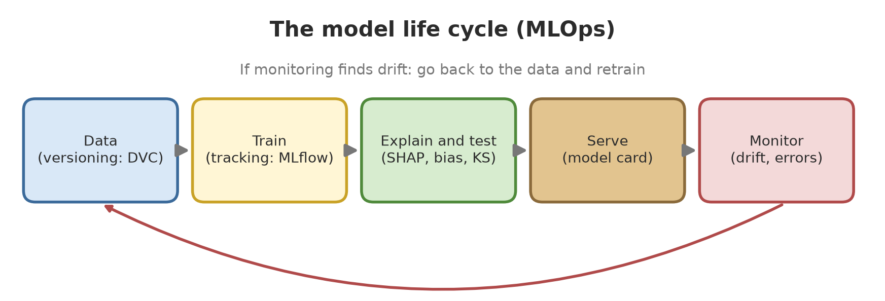
The data in this chapter is the same as in Chapter 54: fictitious land plots. A copy of make_data.py sits in this chapter’s folder so the chapter stands alone. All numbers are examples.
Feature importance: beware of the built-in measure
In Chapter 54 we read feature_importances_ from a random forest. That measure (based on the drop in impurity, how mixed-up the classes in a tree node are) has a weakness: when two features are correlated, the value is split between them. Permutation importance measures how much accuracy drops on the test data when one column is shuffled: if the column matters, accuracy plunges.
We prove it by adding a feature elevation_ft: the same elevation in feet (an exact copy of elevation_m).
01_permutation_importance.py
# Chapter 58 - Feature importance: random forest built-in vs permutation (on test data)
import numpy as np
from sklearn.ensemble import RandomForestClassifier
from sklearn.inspection import permutation_importance
from sklearn.model_selection import train_test_split

from make_data import FEATURES, make_land

df = make_land()
# Add the feature "elevation_ft" = elevation in feet: an almost exact copy of elevation_m (perfectly correlated)
df["elevation_ft"] = df["elevation_m"] * 3.28084
columns = FEATURES + ["elevation_ft"]
X_train, X_test, y_train, y_test = train_test_split(df[columns], df["land_class"], test_size=0.3, random_state=42, stratify=df["land_class"])
model = RandomForestClassifier(n_estimators=200, random_state=42, n_jobs=1).fit(X_train, y_train)
print("Test accuracy:", round(model.score(X_test, y_test), 3))

perm = permutation_importance(model, X_test, y_test, n_repeats=10, random_state=42, n_jobs=1)
print("\nfeature              | built-in RF (impurity) | permutation (accuracy drop)")
for i in np.argsort(-model.feature_importances_):
    print(f"{columns[i]:20s} | {model.feature_importances_[i]:22.3f} | {perm.importances_mean[i]:.3f} +- {perm.importances_std[i]:.3f}")
Test accuracy: 0.881
feature | built-in RF (impurity) | permutation (accuracy drop)
ndvi | 0.418 | 0.333 +- 0.022
elevation_ft | 0.199 | 0.039 +- 0.009
elevation_m | 0.176 | 0.032 +- 0.008
slope_degrees | 0.146 | 0.102 +- 0.012
rainfall_mm | 0.061 | 0.005 +- 0.007Elevation shows up twice (elevation_ft 0.199 and elevation_m 0.176 by the built-in measure), although the information is one and the same. Permutation shows something similar: shuffling one copy lowers accuracy by only 0.039 or 0.032, because the model can still use the other copy. The lesson: before concluding “this feature is not important”, check whether it has a twin.
SHAP: each feature’s contribution to each prediction
SHAP (SHapley Additive exPlanations) splits the difference between one plot’s prediction and the average prediction into a contribution from each feature, using an idea from game theory (sharing a “prize” fairly among “players”). For tree-based models, shap.TreeExplainer computes it quickly and exactly. The SHAP documentation (read 2026-10-10) states that the SHAP values plus the base value (expected_value) add up to the model output, and that scikit-learn random forests are supported.
02_shap_rf.py
# Chapter 58 - SHAP: explaining a random forest prediction per plot, and proof that the explanation "adds up"
import numpy as np
import shap
from sklearn.ensemble import RandomForestClassifier
from sklearn.model_selection import train_test_split

from make_data import FEATURES, make_land

df = make_land()
X_train, X_test, y_train, y_test = train_test_split(df[FEATURES], df["land_class"], test_size=0.3, random_state=42, stratify=df["land_class"])
model = RandomForestClassifier(n_estimators=100, max_depth=8, random_state=42, n_jobs=1).fit(X_train, y_train)
classes = list(model.classes_)

explainer = shap.TreeExplainer(model)
sv = explainer(X_test.iloc[:100])                       # Explanation object: values (plot, feature, class)
print("Shape of SHAP values (plot, feature, class):", sv.values.shape)

# One plot: why did the model answer that way?
i = 0
proba = model.predict_proba(X_test.iloc[[i]])[0]
k = int(np.argmax(proba))
print(f"\nTest plot #{i}: true class = {y_test.iloc[i]}, prediction = {classes[k]} (probability {proba[k]:.2f})")
print("Feature values:", X_test.iloc[i].round(2).to_dict())
print(f"Base probability of class '{classes[k]}' (training-data average): {sv.base_values[i, k]:.3f}")
for name, value in sorted(zip(FEATURES, sv.values[i, :, k]), key=lambda p: -abs(p[1])):
    print(f"  {name:20s} {value:+.3f}")
print("Base + sum of contributions =", round(sv.base_values[i, k] + sv.values[i, :, k].sum(), 3), "| model probability =", round(proba[k], 3))

# Global picture: mean |SHAP| per feature for the class 'forest'
kf = classes.index("forest")
importance = np.abs(sv.values[:, :, kf]).mean(axis=0)
print("\nMean |SHAP| for class 'forest':")
for name, value in sorted(zip(FEATURES, importance), key=lambda p: -p[1]):
    print(f"  {name:20s} {value:.3f}")
Shape of SHAP values (plot, feature, class): (100, 4, 4)
Test plot #0: true class = rice_field, prediction = rice_field (probability 0.77)
Feature values: {'ndvi': 0.48, 'elevation_m': 208.0, 'slope_degrees': 0.1, 'rainfall_mm': 2225.0}
Base probability of class 'rice_field' (training-data average): 0.270
ndvi +0.307
slope_degrees +0.219
rainfall_mm -0.045
elevation_m +0.020
Base + sum of contributions = 0.771 | model probability = 0.771
Mean |SHAP| for class 'forest':
elevation_m 0.131
slope_degrees 0.098
ndvi 0.067
rainfall_mm 0.006- The shape
(100, 4, 4): 100 plots, 4 features, 4 classes. Each class has its own explanation. - Test plot #0 (actually
rice_field) is predicted asrice_fieldwith probability 0.77. The base probability of the rice-field class is only 0.270. NDVI 0.48 adds +0.307 and slope 0.1 degrees adds +0.219; rainfall pulls slightly down (-0.045) and elevation barely matters (+0.020). - The proof:
0.270 + 0.307 + 0.219 - 0.045 + 0.020= 0.771, equal to the model’s probability (0.771). The SHAP explanation really adds up to the prediction. - Globally, for the class
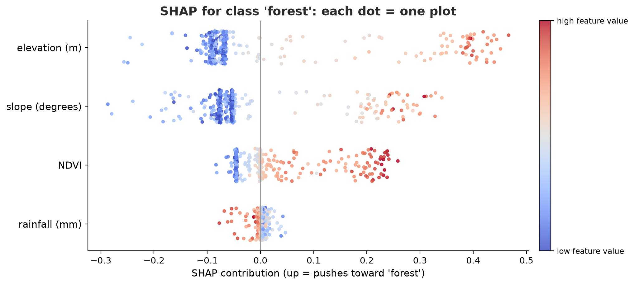
forest: elevation (mean |SHAP| 0.131) and slope (0.098) matter most. Compare this with the RF default in Chapter 54, which put NDVI on top; different measures answer different questions (here: influence on the forest class only).
LIME: random neighbours and a simple model
LIME explains one prediction in another way: it makes thousands of “neighbour” plots by randomly perturbing the features around that plot, asks the real model to guess them, then fits a simple linear model to the results. The coefficients of that simple model are the explanation. We run it three times with different LIME randomness. (Here we ask about the class plantation.)
03_lime.py
# Chapter 58 - LIME: explaining ONE prediction with a simple model around that point
import pandas as pd
from lime.lime_tabular import LimeTabularExplainer
from sklearn.ensemble import RandomForestClassifier
from sklearn.model_selection import train_test_split

from make_data import FEATURES, make_land

df = make_land()
X_train, X_test, y_train, y_test = train_test_split(df[FEATURES], df["land_class"], test_size=0.3, random_state=42, stratify=df["land_class"])
model = RandomForestClassifier(n_estimators=100, max_depth=8, random_state=42, n_jobs=1).fit(X_train, y_train)

def predict(array):                                       # LIME sends NumPy arrays; our model was trained on a DataFrame
    return model.predict_proba(pd.DataFrame(array, columns=FEATURES))


k = list(model.classes_).index("plantation")
for seed in (42, 1, 2):                                   # run three times with different LIME randomness
    explainer = LimeTabularExplainer(X_train.values, feature_names=FEATURES, class_names=list(model.classes_),
                                     discretize_continuous=True, random_state=seed)
    explanation = explainer.explain_instance(X_test.values[0], predict, num_features=4, num_samples=2000, labels=[k])
    print(f"Test plot #0, class 'plantation', LIME random_state = {seed}  (local model R2 = {explanation.score:.2f})")
    for rule, weight in explanation.as_list(label=k):
        print(f"  {rule:45s} {weight:+.3f}")
Test plot #0, class 'plantation', LIME random_state = 42 (local model R2 = 0.03)
0.38 < ndvi <= 0.61 +0.074
slope_degrees <= 1.20 -0.055
114.00 < elevation_m <= 238.50 +0.008
2103.50 < rainfall_mm <= 2243.00 +0.003
Test plot #0, class 'plantation', LIME random_state = 1 (local model R2 = 0.03)
slope_degrees <= 1.20 -0.068
0.38 < ndvi <= 0.61 +0.057
114.00 < elevation_m <= 238.50 +0.022
2103.50 < rainfall_mm <= 2243.00 -0.009
Test plot #0, class 'plantation', LIME random_state = 2 (local model R2 = 0.02)
slope_degrees <= 1.20 -0.049
0.38 < ndvi <= 0.61 +0.046
2103.50 < rainfall_mm <= 2243.00 +0.018
114.00 < elevation_m <= 238.50 -0.004The explanations hold a consistent message: 0.38 < ndvi <= 0.61 pushes toward plantation, while a nearly flat plot (slope_degrees <= 1.20) pushes away from it. This fits SHAP, where NDVI 0.48 and a slope of 0.1 degrees pushed the model toward rice field. But look at the warning signs:
- The numbers differ from run to run (the NDVI weight is +0.074, +0.057, +0.046), the order of the top two features swaps, and the weak features even flip sign (elevation +0.008, +0.022, -0.004). LIME is unstable because it uses random samples.
- The local model’s R² is only 0.02 to 0.03: the simple model can barely imitate the real model around this plot. The explanation cannot be trusted as fine detail.
- SHAP, by contrast, is exact for trees and adds up to the prediction. For tree-based models, prefer SHAP; LIME is useful for models that have no dedicated explainer, used with skepticism and with a check of R².
Partial dependence: the shape of a relationship
Partial dependence answers “if this feature is shifted, how does the average prediction change?” by replacing the value of one feature in all rows and then averaging the predictions.
04_pdp.py
# Chapter 58 - Partial dependence: how the average prediction changes when ONE feature is shifted
import numpy as np
from sklearn.ensemble import RandomForestRegressor
from sklearn.inspection import partial_dependence

from make_data import FEATURES, make_land

df = make_land()
rice = df[df["land_class"] == "rice_field"].copy()
rng = np.random.default_rng(7)
rice["yield_kg_ha"] = (4000 + 5000 * np.sin(np.pi * rice["ndvi"].clip(0, 1))
                       + 0.8 * (rice["rainfall_mm"] - 2200) + rng.normal(0, 250, len(rice))).round(0)
columns = ["ndvi", "rainfall_mm", "elevation_m"]
model = RandomForestRegressor(n_estimators=200, random_state=42, n_jobs=1).fit(rice[columns], rice["yield_kg_ha"])

for feature in ["ndvi", "rainfall_mm"]:
    pd_ = partial_dependence(model, rice[columns], [feature], grid_resolution=6)
    print(f"\nPartial dependence of yield on {feature}:")
    for value, pred in zip(pd_["grid_values"][0], pd_["average"][0]):
        print(f"  {feature} = {value:8.2f}  ->  average yield = {pred:7.0f} kg/ha")
Partial dependence of yield on ndvi:
  ndvi =     0.25  ->  average yield =    7259 kg/ha
  ndvi =     0.33  ->  average yield =    8175 kg/ha
  ndvi =     0.41  ->  average yield =    8708 kg/ha
  ndvi =     0.49  ->  average yield =    8830 kg/ha
  ndvi =     0.57  ->  average yield =    8759 kg/ha
  ndvi =     0.65  ->  average yield =    8185 kg/ha

Partial dependence of yield on rainfall_mm:
  rainfall_mm =  1811.42  ->  average yield =    8372 kg/ha
  rainfall_mm =  1929.86  ->  average yield =    8404 kg/ha
  rainfall_mm =  2048.30  ->  average yield =    8490 kg/ha
  rainfall_mm =  2166.73  ->  average yield =    8524 kg/ha
  rainfall_mm =  2285.17  ->  average yield =    8653 kg/ha
  rainfall_mm =  2403.61  ->  average yield =    8675 kg/ha
Rice yield (example numbers) rises from 7,259 kg/ha at NDVI 0.25 to a peak of 8,830 at NDVI 0.49, then falls to 8,185 at 0.65: the relationship is curved, just as we built it in Chapter 54. Rainfall raises yield only slowly, from 8,372 to 8,675. A relationship like this is not visible from feature_importances_ numbers alone.
A model explanation tells you what the model does, not what happens in nature. “High NDVI pushes the forest prediction” does not mean raising NDVI would turn the plot into forest. Cause and effect need a study design, not just a model (Chapters 26-27).
MLflow: a notebook for experiments
After dozens of experiments, who remembers which model used which parameters and scored what? MLflow (tracking) logs the parameters, metrics, and files of each experiment (run) to local storage or a server. We use a SQLite database in the _tmp/ folder, with no server at all.
05_mlflow.py
# Chapter 58 - MLflow: logging experiments (parameters, metrics, model) to a local folder, no server
import logging
import shutil
from pathlib import Path

import mlflow
from sklearn.ensemble import RandomForestClassifier
from sklearn.model_selection import GroupKFold, cross_val_score

from make_data import FEATURES, make_land

logging.disable(logging.INFO)                         # hide MLflow INFO logs, which contain timestamps
folder = Path(__file__).parent / "_tmp" / "mlflow_local"
shutil.rmtree(folder, ignore_errors=True)
folder.mkdir(parents=True)
mlflow.set_tracking_uri(f"sqlite:///{(folder / 'mlflow.db').as_posix()}")        # local SQLite database
mlflow.set_experiment("land-cover")

df = make_land()
for n_trees, depth in [(50, 4), (100, 8), (200, 12)]:
    with mlflow.start_run(run_name=f"rf_{n_trees}_{depth}"):
        model = RandomForestClassifier(n_estimators=n_trees, max_depth=depth, random_state=42, n_jobs=1)
        scores = cross_val_score(model, df[FEATURES], df["land_class"], groups=df["block"], cv=GroupKFold(n_splits=4))
        mlflow.log_params({"n_estimators": n_trees, "max_depth": depth, "validation": "GroupKFold block"})
        mlflow.log_metric("block_accuracy", float(scores.mean()))
        mlflow.log_metric("std_dev", float(scores.std()))

results = mlflow.search_runs(experiment_names=["land-cover"], order_by=["metrics.block_accuracy DESC"])
print("Number of runs logged:", len(results))
print(results[["tags.mlflow.runName", "params.n_estimators", "params.max_depth", "metrics.block_accuracy"]]
      .round(3).to_string(index=False))
print("\nMLflow database file exists:", (folder / "mlflow.db").exists())
Number of runs logged: 3
tags.mlflow.runName params.n_estimators params.max_depth metrics.block_accuracy
rf_200_12 200 12 0.889
rf_100_8 100 8 0.884
rf_50_4 50 4 0.876
MLflow database file exists: TrueThree runs (50, 100, and 200 trees) were logged, and search_runs sorts them by highest block accuracy: 0.889 for 200 trees with depth 12. On your computer, mlflow ui --backend-store-uri sqlite:///... opens a web interface to compare them (not run in this book). We could not read the MLflow documentation on storage options today, so this book only states that the SQLite route works in the installed MLflow version.
Also log the data version and the code version (Git hash) as parameters. Without them, “the 0.889 model” cannot be reproduced three months from now.
DVC: versions for data
Git is great for code but poor for big data files. DVC (Data Version Control) stores the data somewhere else (a shared disk, the cloud) and puts only a small .dvc file, holding the data’s fingerprint (hash), into Git. Changing the data changes its fingerprint, so Git records the data version together with the code version.
DVC cannot yet be installed on Python 3.14, the version used in this book: pip fails to resolve its dependencies (tried 2026-10-10). We installed it in a separate Python 3.12 environment (DVC 3.67.1) and captured the real output once; this text uses that saved output (@statis), so the script below is not re-run when the book is built.
09_dvc_data_versions.py
# Chapter 58 - DVC: versioning data like Git does for big files (run through the dvc command in a temporary folder)
import os
import shutil
import stat
import subprocess
from pathlib import Path

work = Path(__file__).parent / "_tmp" / "demo_dvc"


def force_delete(func, path, error):                    # DVC creates read-only cache files on Windows; allow writing first, then delete
    os.chmod(path, stat.S_IWRITE)
    func(path)


if work.exists():
    shutil.rmtree(work, onexc=force_delete)
work.mkdir(parents=True)
os.environ["DVC_NO_ANALYTICS"] = "1"


def dvc(*args):
    result = subprocess.run(["dvc", *args], cwd=work, capture_output=True, text=True)
    print("$ dvc", *args)
    print((result.stdout + result.stderr).strip())


(work / "land.csv").write_text("plot,ndvi\n1,0.81\n2,0.35\n3,0.62\n", encoding="utf-8")
dvc("init", "--no-scm")                    # --no-scm: no Git, for the demo only
dvc("add", "land.csv")
print("\nContents of land.csv.dvc (the small file that goes into Git):")
print((work / "land.csv.dvc").read_text(encoding="utf-8"))
dvc("status")
(work / "land.csv").write_text("plot,ndvi\n1,0.81\n2,0.35\n3,0.62\n4,0.48\n", encoding="utf-8")   # data changes
print("\nAfter the data changed:")
dvc("status")
$ dvc init --no-scm
Initialized DVC repository.
What's next?
------------
- Check out the documentation: <https://dvc.org/doc>
- Get help and share ideas: <https://dvc.org/chat>
- Star us on GitHub: <https://github.com/treeverse/dvc>
$ dvc add land.csv
Contents of land.csv.dvc (the small file that goes into Git):
outs:
- md5: d8d36037f5f60a6c74355722425a1c74
size: 35
hash: md5
path: land.csv
$ dvc status
Data and pipelines are up to date.
After the data changed:
$ dvc status
land.csv.dvc:
changed outs:
modified: land.csvdvc init --no-scmsets up DVC without Git (for the demo only; in a real project you use Git).dvc add land.csvcomputes the md5 hashd8d36037...and writesland.csv.dvc. This small file is what yougit add.dvc statussays “up to date” and then, after we add one row of data, reportsmodified: land.csv: DVC noticed the data changed from its hash.- The commands
dvc pushanddvc pull(to send data to remote storage) are not tried here.
Monitoring a model: drift
A model is trained on a snapshot of the past. The world changes: sensors age, a long dry season arrives, a policy changes planting. A shift in the distribution of the input data is called data drift. The simplest way to detect it: compare the distribution of each feature between the training data and the new data with the Kolmogorov-Smirnov test (scipy.stats.ks_2samp). A small p-value means the two distributions very likely differ.
06_drift_ks.py
# Chapter 58 - Monitoring drift: is the new data still "of the same kind" as the training data? (Kolmogorov-Smirnov test)
import numpy as np
from scipy.stats import ks_2samp

from make_data import FEATURES, make_land

everything = make_land(n=2400, seed=42)
shuffled = np.random.default_rng(0).permutation(len(everything))
train = everything.iloc[shuffled[:1200]]              # data from when the model was trained
safe = everything.iloc[shuffled[1200:1800]]           # new data from the same process
shifted = everything.iloc[shuffled[1800:]].copy()     # new data, but field conditions changed
shifted["ndvi"] = (shifted["ndvi"] - 0.08).round(3)                      # ageing sensor / dry season: NDVI drops by 0.08
shifted["rainfall_mm"] = shifted["rainfall_mm"] * 0.85                   # rainfall 15% lower

print("feature              | normal new data (p) | shifted new data (p)")
for f in FEATURES:
    p_safe = ks_2samp(train[f], safe[f]).pvalue
    p_shift = ks_2samp(train[f], shifted[f]).pvalue
    flag = "  <- DRIFT" if p_shift < 0.01 else ""
    print(f"{f:20s} | {p_safe:19.3f} | {p_shift:20.4g}{flag}")


def psi(a, b, k=10):
    """Population Stability Index: <0.1 stable, 0.1-0.25 watch, >0.25 big change (industry rule of thumb)."""
    edges = np.quantile(a, np.linspace(0, 1, k + 1))
    edges[0], edges[-1] = -np.inf, np.inf
    pa = np.histogram(a, edges)[0] / len(a) + 1e-6
    pb = np.histogram(b, edges)[0] / len(b) + 1e-6
    return float(((pb - pa) * np.log(pb / pa)).sum())


print("\nPSI NDVI, normal data :", round(psi(train["ndvi"], safe["ndvi"]), 3))
print("PSI NDVI, shifted data:", round(psi(train["ndvi"], shifted["ndvi"]), 3))
feature | normal new data (p) | shifted new data (p)
ndvi | 0.412 | 1.368e-05 <- DRIFT
elevation_m | 0.995 | 0.679
slope_degrees | 0.882 | 0.4124
rainfall_mm | 0.595 | 1.046e-132 <- DRIFT
PSI NDVI, normal data : 0.01
PSI NDVI, shifted data: 0.166- “Normal” new data (drawn from the same map) has a p-value of 0.412 for NDVI and 0.995 for elevation: no drift, as expected.
- After NDVI is lowered by 0.08 and rainfall is cut by 15%, the KS test flags both (p = 1.4 x 10^-5 and 1 x 10^-132). Elevation and slope did not change and are not flagged.
- PSI (population stability index) sums up the shift in one number: 0.010 (normal) vs 0.166 (shifted). The thresholds “below 0.1 stable, 0.1 to 0.25 watch, above 0.25 big change” are an industry rule of thumb, not a formal standard.
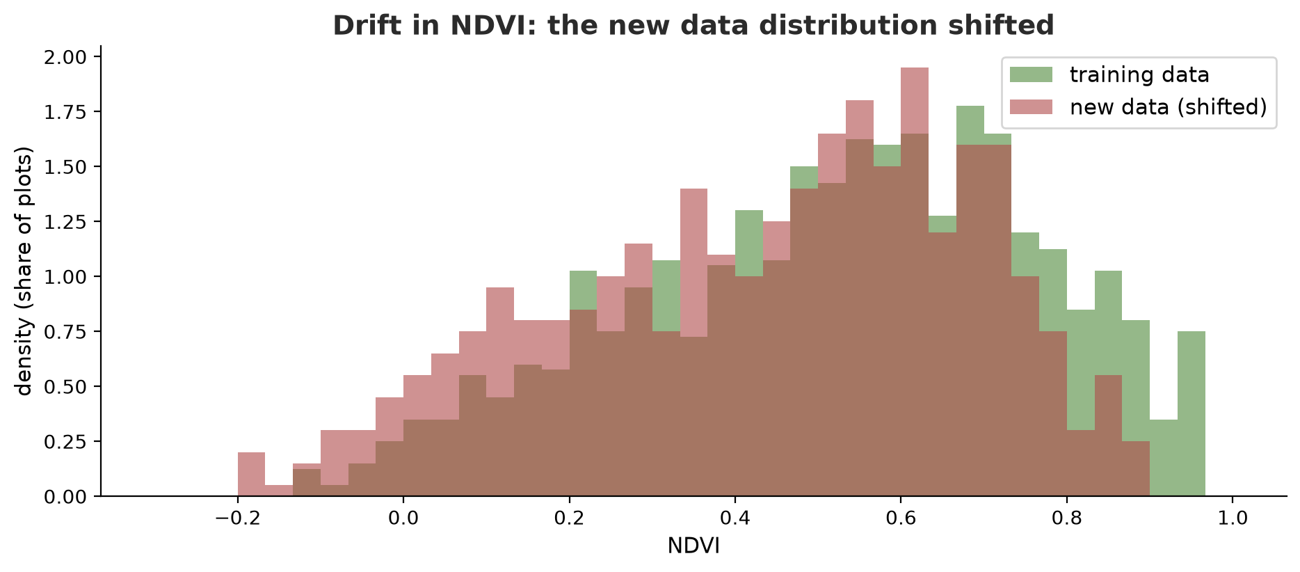
The KS test with big data is very sensitive: a tiny difference with no impact can produce a minuscule p-value. Complement it with a measure of how large the shift is (PSI, difference of means) and, when available, the real performance of the model on recent labelled data. Drift in a feature does not automatically mean the model is bad.
Prediction uncertainty
A model that says “yield 8,696 kg/ha” with no range sounds more sure than it should. Two ways to give a range:
- Spread of the trees: each tree in a random forest gives its own prediction; the spread shows how much they disagree. Easy, but the coverage is not guaranteed.
- Conformal prediction (the split version): set aside calibration data, measure the model’s real errors on it, and use a quantile of the errors as the interval width. Assuming the calibration data and the new data are alike, it guarantees coverage of at least about the requested level (here 90%) on average.
07_uncertainty.py
# Chapter 58 - Prediction uncertainty: an interval from the spread of trees, and "conformal prediction" with tested coverage
import numpy as np
from sklearn.ensemble import RandomForestRegressor
from sklearn.model_selection import train_test_split

from make_data import make_land

df = make_land()
rng = np.random.default_rng(7)
rice = df[df["land_class"] == "rice_field"].copy()
rice["yield_kg_ha"] = (4000 + 5000 * np.sin(np.pi * rice["ndvi"].clip(0, 1))
                       + 0.8 * (rice["rainfall_mm"] - 2200) + rng.normal(0, 250, len(rice))).round(0)
columns = ["ndvi", "rainfall_mm", "elevation_m"]
X_rest, X_test, y_rest, y_test = train_test_split(rice[columns], rice["yield_kg_ha"], test_size=0.3, random_state=1)
X_train, X_cal, y_train, y_cal = train_test_split(X_rest, y_rest, test_size=0.4, random_state=1)   # separate calibration set
model = RandomForestRegressor(n_estimators=200, random_state=42, n_jobs=1).fit(X_train, y_train)

# 1) Spread of the 200 trees' predictions for one plot
all_trees = np.array([p.predict(X_test.iloc[[0]].values)[0] for p in model.estimators_])
print(f"Test plot #0: forest prediction = {model.predict(X_test.iloc[[0]])[0]:.0f} kg/ha, actual = {y_test.iloc[0]:.0f}")
print(f"  the trees disagree: 10%-90% = {np.percentile(all_trees, 10):.0f} to {np.percentile(all_trees, 90):.0f}")

# 2) Split conformal prediction: measure the real error on calibration data, use it as the interval width
errors = np.abs(y_cal - model.predict(X_cal))
alpha = 0.1                                                                 # target coverage 90%
n = len(errors)
q = np.quantile(errors, min(1.0, np.ceil((n + 1) * (1 - alpha)) / n))
pred = model.predict(X_test)
covered = np.mean((y_test >= pred - q) & (y_test <= pred + q))
print(f"\nConformal: interval width = +-{q:.0f} kg/ha (from {n} calibration plots)")
print(f"Coverage on {len(y_test)} test plots (target 90%): {covered:.0%}")

# The 5%-95% interval from the tree spread is not guaranteed to meet the coverage
lo, hi = [], []
for x in X_test.values:
    ps = np.array([p.predict(x.reshape(1, -1))[0] for p in model.estimators_])
    lo.append(np.percentile(ps, 5)), hi.append(np.percentile(ps, 95))
print("Coverage of the 5%-95% tree-spread interval (nominal 90%):", f"{np.mean((y_test >= lo) & (y_test <= hi)):.0%}")
Test plot #0: forest prediction = 8696 kg/ha, actual = 8692
the trees disagree: 10%-90% = 8389 to 9273
Conformal: interval width = +-564 kg/ha (from 92 calibration plots)
Coverage on 98 test plots (target 90%): 97%
Coverage of the 5%-95% tree-spread interval (nominal 90%): 82%- Plot #0: prediction 8,696, actual 8,692; the trees disagree over a range of 8,389 to 9,273 (10th-90th percentile).
- Conformal: an interval of ±564 kg/ha from 92 calibration plots, with coverage on 98 test plots of 97% (target at least 90%). Coverage above the target is normal: the guarantee is a lower bound on average, and a small sample can make the interval conservative.
- The 5%-95% interval from the tree spread, labelled “90%”, covers only 82% of the actual values: it is overconfident. Without a coverage test like this, we would not know which interval is honest.
Bias, privacy, and the model card
Bias here means the model works badly for certain groups without anyone noticing, because the overall accuracy hides it. Check performance per group: per class, per region, per season, per group of landowners if the data exists. Privacy: coordinates of privately owned plots can reveal who the owner is; blur them before sharing the data. A model card is a short document (proposed by researchers as a model documentation practice) covering a model’s purpose, data, evaluation, weaknesses, and limits of use.
08_bias_and_model_card.py
# Chapter 58 - Bias across regions, blurring coordinates (privacy), and a model card
import json
from pathlib import Path

import numpy as np
import pandas as pd
from sklearn.ensemble import RandomForestClassifier
from sklearn.model_selection import GroupKFold, cross_val_predict

from make_data import FEATURES, make_land

df = make_land()
model = RandomForestClassifier(n_estimators=100, max_depth=8, random_state=42, n_jobs=1)
df["prediction"] = cross_val_predict(model, df[FEATURES], df["land_class"], groups=df["block"], cv=GroupKFold(n_splits=4))
df["correct"] = df["prediction"] == df["land_class"]

# 1) Performance per group: overall accuracy can hide a group that is treated badly
print("Overall accuracy:", round(df["correct"].mean(), 3))
print("\nAccuracy per true class (recall):")
print(df.groupby("land_class")["correct"].agg(["mean", "size"]).round(3).rename(columns={"mean": "accuracy", "size": "count"}).to_string())
df["region"] = np.where(df["x"] < 500, "west", "east")
print("\nAccuracy per region:")
print(df.groupby("region")["correct"].agg(["mean", "size"]).round(3).rename(columns={"mean": "accuracy", "size": "count"}).to_string())

# 2) Privacy: coordinates of privately owned plots can be blurred before the data is shared
public = df[["x", "y"]].copy()
public["x"], public["y"] = (public["x"] // 100) * 100, (public["y"] // 100) * 100       # rounded to a 100 m cell
print("\nUnique points before blurring:", len(df[["x", "y"]].drop_duplicates()), "| after:", len(public.drop_duplicates()))

# 3) Model card: a short document about the model, built from the real numbers of the experiment
card = {
    "name": "Land cover classification (random forest, book example)",
    "purpose": "Map four land classes from NDVI, elevation, slope, and rainfall on FICTITIOUS data",
    "data": f"{len(df)} fictitious plots, 1000 x 1000 m map, 4 classes",
    "evaluation": f"GroupKFold 4 folds based on 250 m blocks; accuracy {df['correct'].mean():.3f}",
    "weakness": "weakest class: " + df.groupby("land_class")["correct"].mean().idxmin(),
    "not_for": ["legal decisions or sanctions", "areas with different sensors or seasons without re-validation"],
    "monitoring": "KS test and PSI on NDVI and rainfall every month",
}
file = Path(__file__).parent / "_tmp" / "model_card.json"
file.parent.mkdir(exist_ok=True)
file.write_text(json.dumps(card, indent=2, ensure_ascii=False), encoding="utf-8")
print("\nModel card contents:")
print(file.read_text(encoding="utf-8"))
Overall accuracy: 0.884
Accuracy per true class (recall):
accuracy count
land_class
forest 0.939 198
plantation 0.753 146
rice_field 0.837 326
settlement 0.928 530
Accuracy per region:
accuracy count
region
east 0.863 598
west 0.905 602
Unique points before blurring: 1200 | after: 100
Model card contents:
{
"name": "Land cover classification (random forest, book example)",
"purpose": "Map four land classes from NDVI, elevation, slope, and rainfall on FICTITIOUS data",
"data": "1200 fictitious plots, 1000 x 1000 m map, 4 classes",
"evaluation": "GroupKFold 4 folds based on 250 m blocks; accuracy 0.884",
"weakness": "weakest class: plantation",
"not_for": [
"legal decisions or sanctions",
"areas with different sensors or seasons without re-validation"
],
"monitoring": "KS test and PSI on NDVI and rainfall every month"
}- An overall accuracy of 0.884 sounds good, but the class
plantationis only 0.753 whileforestis 0.939. A map used for plantation policy will be wrong most often. - West region 0.905 vs east 0.863: slightly worse in the east. A gap this small could be chance; what matters is to check.
- 1,200 unique points become 100 cells after the coordinates are rounded to 100 m. Blurring reduces the risk, but does not guarantee anonymity if other data can be matched.
- The model card is built from the real numbers of the experiment, complete with a “not for” list (legal decisions or sanctions) and a monitoring plan.
Running Project A3: a model you can stand behind
This project is not a new script but a habit: for every Series A3 model, prepare the following five things before handing the map to users.
| User’s question | Tool in this chapter |
|---|---|
| “Why is this plot like this?” | SHAP (script 02), partial dependence (04) |
| “Which experiment was used, can it be repeated?” | MLflow (05), DVC (09) |
| “Will it still be valid next year?” | KS and PSI (06) |
| “How sure are you?” | Conformal (07) |
| “Is it fair and safe?” | Accuracy per group, coordinate blurring, model card (08) |
Exercises
- In
02_shap_rf.py, replacei = 0with another plot and write a one-sentence explanation from its SHAP numbers. - In
03_lime.py, raisenum_samplesfrom 2000 to 20000. Do the local R² and the stability between runs improve? - In
06_drift_ks.py, reduce NDVI by only 0.01. Does KS still flag drift? What does the result mean? - Challenge: change
07_uncertainty.pyto try the targetsalpha = 0.2(80% coverage) and 0.05 (95%). Does the real coverage follow the target?
Chapter Summary
- The built-in feature importance can mislead when features are correlated; try permutation.
- SHAP explains each prediction with contributions that add up; LIME is random and can be unstable; partial dependence shows the shape of a relationship.
- MLflow logs experiments; DVC versions data through hashes.
- Drift: compare the distribution of new data with the training data (KS, PSI), and do not forget to monitor real performance.
- Give uncertainty intervals whose coverage is tested (conformal).
- Check performance per group, blur personal data, and write a model card.
Next, in Chapter 59: all the Series A3 tools meet in the field: forestry, agriculture, fisheries, livestock, and natural resources, from LiDAR to livestock in aerial photos.