Chapter 28 — Qualitative and Mixed Methods: Hearing the Stories, Then Counting Them

Series I3 — Statistics and Modelling

NoteIn this chapter, you will:

• Understand when to use qualitative, quantitative, or mixed methods
• Code interviews into themes with a codebook, then count how often they appear
• Use basic text tools: word frequency, KWIC, TF-IDF, topic modelling, and dictionary-based sentiment
• Understand embeddings as a concept and turn qualitative data into numbers
• Judge the validity, reliability, and ethics of research, then combine stories and numbers in mixed methods

All scripts for this chapter are in the kode/ch28/ folder. On the web version, you can also download them all at once (zip).

Chapters 26 and 27 dealt with numbers. But if you want to know why farmers are reluctant to plant trees on their land, or how fishers cope with the lean season, numbers alone are not enough. You need to hear the stories. Imagine a veterinarian: a cow’s temperature says the cow has a fever, but the keeper’s story (“yesterday my cow refused to eat, and my neighbour lost two animals”) says why and what to look for. Qualitative methods analyse words, meaning, and stories; mixed methods combine both.

WarningWARNING

Ethics note and made-up data. All respondents, interview quotes, and survey numbers in this chapter are fictional, written by the book author for practice, and do not represent any person or village. In real research you must: (1) obtain the respondents’ consent after explaining the purpose and risks (informed consent, ideally written); (2) disguise identities (anonymisation) in data and reports; (3) store recordings and transcripts securely; (4) explain that respondents may stop at any time. For indigenous and local communities, there is also a principle of community consent sought beforehand and without pressure, which you should study from your ethics committee’s guidelines. Also check your institution’s or university’s rules on research permits.

Qualitative, quantitative, or mixed?

	Quantitative	Qualitative
Typical question	How many? How big? Is there a difference?	Why? How? What does it mean?
Data	Numbers (weight, harvest, score 1-5)	Text, stories, observations, documents
Sample	Large, random	Small, chosen on purpose
Main tools	Hypothesis tests, regression (Chapters 26-27)	Theme coding, content analysis
Strength	Can be generalised, measurable	Rich in context, finds the unexpected
Weakness	Shallow on “why”	Hard to generalise, prone to subjectivity

A rule of thumb: quantitative for “how many”, qualitative for “why”, and both when the decision is important. There are three common mixed designs:

• Explanatory sequential: a numeric survey first, then interviews to explain surprising findings.
• Exploratory sequential: interviews first to discover the topics, then a survey to measure how common they are.
• Convergent (parallel): both are collected at the same time and then compared. Our project uses this.

%%{init: {"flowchart": {"diagramPadding": 40}}}%%
flowchart TD
  A["Research question"] --> B["Open<br/>interviews"]
  A --> C["Numeric<br/>survey"]
  B --> D["Theme coding<br/>(Python: text)"]
  C --> E["Statistics<br/>(Python: Ch. 26-27)"]
  D --> F["Joint<br/>display"]
  E --> F
  F --> G["Conclusion<br/>and validation"]

A convergent mixed design: two data tracks collected together, then merged into one conclusion.

Our made-up interview data

We use 24 short fictional interviews: 8 farmers, 8 fishers, 8 livestock keepers. The open question: “What is the biggest change you have felt in the last five years, and how did you deal with it?” Each respondent also filled in a satisfaction score (1 to 5) and an income (million rupiah per month), so we have both a story and numbers for the same person. The data is in kode/ch28/data/interviews.csv.

01_interview_data.py

# Chapter 28 - Reading made-up (fictional) interview data
from pathlib import Path

import pandas as pd

# ETHICS NOTE: all respondents and quotes in this chapter are FICTIONAL, written by the book author.
# In real research you must obtain written informed consent, disguise identities (anonymisation),
# and store recordings securely.
data = pd.read_csv(Path(__file__).parent / "data" / "interviews.csv")

print("Number of respondents:", len(data))
print(data["role"].value_counts().to_string())
print()
print("Average satisfaction (scale 1-5) by role:")
print(data.groupby("role")["satisfaction"].mean().round(2).to_string())
print()
data["word_count"] = data["answer"].str.split().str.len()
print("Answer length (words): min", data["word_count"].min(), " max", data["word_count"].max(),
      " mean", round(data["word_count"].mean(), 1))
print()
for _, row in data.head(3).iterrows():
    print(f"[{row['code']}, {row['role']}, {row['age']} y] {row['answer']}")

Number of respondents: 24
role
farmer              8
fisher              8
livestock keeper    8

Average satisfaction (scale 1-5) by role:
role
farmer              2.75
fisher              2.50
livestock keeper    3.00

Answer length (words): min 21  max 32  mean 26.0

[R01, farmer, 45 y] The rain is unpredictable now. Last year my rice field ran dry right after planting, and the harvest dropped by almost half. I worry it will happen again this year.
[R02, farmer, 52 y] Fertiliser keeps getting more expensive, yet the price of rice drops at harvest time. Middlemen come with cheap offers and we have to sell because we need cash.
[R03, farmer, 38 y] Our farmer group helps. We buy fertiliser together so it is cheaper, and the extension officer visits every month. This year's harvest is good and I am happy.

Each group has 8 people. Average satisfaction: fishers 2.50, farmers 2.75, livestock keepers 3.00. The answers are short, 21 to 32 words (real interviews are far longer). The first three quotes show the variety: drought, a low price from a middleman, and a farmer group that helps.

Theme coding

Coding means attaching a label to pieces of text that talk about the same thing. The label is called a code or theme. The list of themes with their definitions is called a codebook. There are two ways to build it:

• Inductive: themes emerge from the data; you read first, then name the repeating patterns.
• Deductive: themes come from theory or the research question, then are looked for in the data.

In practice researchers mix them: start inductively from part of the transcripts, build a codebook, then apply it deductively to all the data. Python helps with that last step. The simplest way: each theme has a list of keywords.

02_theme_coding.py

# Chapter 28 - Theme coding with a simple codebook
import re
from pathlib import Path

import pandas as pd

data = pd.read_csv(Path(__file__).parent / "data" / "interviews.csv")

# Codebook: theme -> keywords (word beginnings). Built by the researcher after reading part of the data.
codebook = {
    "climate": ["rain", "dry", "weather", "flood", "waves", "lean season"],
    "price_market": ["price", "middlem", "collector", "sell", "margin"],
    "cost_capital": ["capital", "loan", "interest", "expensive", "cost", "diesel", "fertili", "feed"],
    "pest_disease": ["pest", "planthopper", "disease", "vaccine", "died", "bombing"],
    "cooperation": ["group", "cooperat", "working together", "together", "share"],
    "technology_info": ["app", "phone", "video", "information", "training", "extension officer", "guidance"],
    "rules_land": ["permit", "forest area", "evicted", "rules", "zone", "certificate", "officers"],
}


def assign_codes(text):
    """List of themes whose keyword appears in the text (lower case, word beginning)."""
    text = text.lower()
    return [theme for theme, keys in codebook.items()
            if any(re.search(r"\b" + re.escape(k), text) for k in keys)]


data["themes"] = data["answer"].apply(assign_codes)
for theme in codebook:
    data[theme] = data["themes"].apply(lambda items: theme in items)

print("Number of respondents mentioning each theme (out of", len(data), "respondents):")
print(data[list(codebook)].sum().sort_values(ascending=False).to_string())
print()
print("Average themes per respondent:", round(data["themes"].str.len().mean(), 2))
print("Respondents with no theme at all:", int((data["themes"].str.len() == 0).sum()))
print()
for code in ("R01", "R03", "R09"):
    row = data[data["code"] == code].iloc[0]
    print(code, "->", row["themes"])

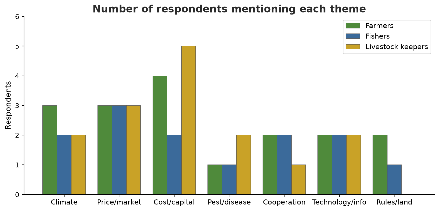
Number of respondents mentioning each theme (out of 24 respondents):
cost_capital       11
price_market        9
climate             7
technology_info     6
cooperation         5
pest_disease        4
rules_land          3

Average themes per respondent: 1.88
Respondents with no theme at all: 0

R01 -> ['climate']
R03 -> ['cost_capital', 'cooperation', 'technology_info']
R09 -> ['climate']

• re.search(r"\b" + word, text) looks for a keyword starting at a word boundary. \b means “word boundary”, learned in Chapter 22.
• The most common theme is cost_capital (11 of 24 respondents), then price_market (9) and climate (7). The rarest theme: rules_land (3).
• On average 1.88 themes per respondent: one answer often talks about several things, so the number of themes is larger than the number of respondents. R03 gets three themes: cost_capital, cooperation, and technology_info.

WarningWARNING

Keyword-based coding is fast and consistent but crude. A keyword like rain also catches “rainfall” and “rainy” (good), but expensive is always counted as cost even when it is about something else, and a person who writes “drought” without the word “dry” is missed. That is why machine results need to be re-read by a human. Treat automatic codes as a fast but careless assistant, not a judge.

Number of respondents mentioning each theme, by role. Costs and capital are mentioned by many groups; land rules are more typical of farmers.

Content analysis: word frequency and KWIC

Content analysis systematically counts and groups elements of text. Two basic tools: word frequency (after removing common words such as “the”, “and”, called stopwords) and KWIC (keyword in context), which shows a keyword with a few words to its left and right so you can see how the word is used.

03_word_frequency.py

# Chapter 28 - Content analysis: word frequency and KWIC (keyword in context)
import re
from collections import Counter
from pathlib import Path

import pandas as pd

data = pd.read_csv(Path(__file__).parent / "data" / "interviews.csv")

COMMON = set("""the and for are but with that this have has had our not was were from its they their them
when which what your you also all can will would one two out into than then too very much many more
some any each just only now last year because while since before after over under again still even
until about there here been being does did done like get got may might must should could every both
off her his him she him how why who whom those these other another such own same""".split())


def words(text):
    return [w for w in re.findall(r"[a-z]+", text.lower()) if w not in COMMON and len(w) > 2]


total = Counter()
for answer in data["answer"]:
    total.update(words(answer))

print("15 most frequent words (after removing common words):")
for word, n in total.most_common(15):
    print(f"  {word:12} {n}")

# KWIC: show the keyword with 4 words to the left and right
print()
print("Context of the word 'price':")
for code, answer in zip(data["code"], data["answer"]):
    tokens = re.findall(r"[A-Za-z]+", answer)
    for i, t in enumerate(tokens):
        if t.lower() == "price":
            left = " ".join(tokens[max(0, i - 4):i])
            right = " ".join(tokens[i + 1:i + 5])
            print(f"  {code}: ...{left} [{t}] {right}...")
            break

15 most frequent words (after removing common words):
  fish         9
  price        7
  helps        6
  feed         6
  hard         5
  together     4
  good         4
  high         4
  costs        4
  often        4
  dry          3
  harvest      3
  dropped      3
  worry        3
  getting      3

Context of the word 'price':
  R02: ...more expensive yet the [price] of rice drops at...
  R11: ...fish at a stable [price] and provides ice Since...
  R12: ...The collector sets the [price] and often squeezes us...
  R13: ...are fresher and the [price] is better...
  R17: ...very expensive and the [price] keeps rising My cows...
  R21: ...up and the selling [price] is good That cooperation...

The most frequent words: fish (9), price (7), helps (6), feed (6). Frequency gives a hint, not an answer: “price” appears often, but KWIC shows the contexts are very different. R02: the price of rice drops (bad); R11: a stable price through the cooperative (good); R17: the price of feed keeps rising. Same word, opposite meanings. That is why content analysis must not stop at counts.

In policy document analysis (for example forest management regulations), the same tools are used: count keywords such as “community”, “permit”, and “sanction”, then compare with KWIC to see who is named as the subject and who as the object. Discourse analysis goes further: it asks how word choices shape a picture of who has authority and who is to blame. This part is more careful reading than counting, and Python only helps find the passages worth reading.

TF-IDF: distinctive words

A frequent word is not necessarily distinctive. “Fish” appears often among fishers, but what sets fishers apart from farmers? TF-IDF (term frequency-inverse document frequency) gives a high score to words that are frequent in this document but rare in the others. Here, each role group is joined into one “document”.

04_tfidf.py

# Chapter 28 - TF-IDF: words that are distinctive for each group of respondents
from pathlib import Path

import pandas as pd
from sklearn.feature_extraction.text import TfidfVectorizer

data = pd.read_csv(Path(__file__).parent / "data" / "interviews.csv")

COMMON = """the and for are but with that this have has had our not was were from its they their them
when which what your you also all can will would one two out into than then too very much many more
some any each just only now last year because while since before after over under again still even
until about there here been being does did done like get got may might must should could every both
off her his him she how why who whom those these other another such own same""".split()

# Join all answers per role into one "document"
per_role = data.groupby("role")["answer"].apply(" ".join)

vectoriser = TfidfVectorizer(stop_words=COMMON, token_pattern=r"[a-z]{3,}", lowercase=True)
matrix = vectoriser.fit_transform(per_role)
words = vectoriser.get_feature_names_out()

print("Matrix size (roles x words):", matrix.shape)
for i, role in enumerate(per_role.index):
    scores = pd.Series(matrix[i].toarray()[0], index=words).sort_values(ascending=False)
    print(f"{role:17}", ", ".join(f"{w} ({s:.2f})" for w, s in scores.head(5).items()))

Matrix size (roles x words): (3, 230)
farmer            harvest (0.28), fertiliser (0.19), middlemen (0.19), planting (0.19), land (0.19)
fisher            fish (0.67), price (0.18), fishing (0.15), reef (0.15), income (0.15)
livestock keeper  feed (0.51), cattle (0.17), fall (0.17), livestock (0.17), thin (0.17)

The matrix is 3 roles x 230 words. Distinctive for fishers: fish, price, fishing, reef, income. Farmers: harvest, fertiliser, middlemen, planting, land. Livestock keepers: feed, cattle, livestock. A high TF-IDF score means “a distinguishing mark of this group”. It is a quick way to draw an initial picture before reading in depth.

Topic modelling: topics from a pile of text

When the text runs to thousands of pages, reading it all is impossible. Topic modelling looks for hidden topics: groups of words that tend to appear together. We use NMF (non-negative matrix factorization) from scikit-learn on the TF-IDF matrix. A popular alternative is LatentDirichletAllocation (LDA) in the same library; both are used similarly. We choose the number of topics (n_components) ourselves.

05_topics_nmf.py

# Chapter 28 - Topic modelling with NMF (scikit-learn)
from pathlib import Path

import numpy as np
import pandas as pd
from sklearn.decomposition import NMF
from sklearn.feature_extraction.text import TfidfVectorizer

data = pd.read_csv(Path(__file__).parent / "data" / "interviews.csv")

COMMON = """the and for are but with that this have has had our not was were from its they their them
when which what your you also all can will would one two out into than then too very much many more
some any each just only now last year because while since before after over under again still even
until about there here been being does did done like get got may might must should could every both
off her his him she how why who whom those these other another such own same""".split()

vectoriser = TfidfVectorizer(stop_words=COMMON, token_pattern=r"[a-z]{3,}", min_df=2)
X = vectoriser.fit_transform(data["answer"])
words = vectoriser.get_feature_names_out()
print("Words used (appearing in >= 2 answers):", len(words))

model = NMF(n_components=4, init="nndsvd", random_state=42, max_iter=500)
doc_weights = model.fit_transform(X)          # respondents x topics

for t, component in enumerate(model.components_):
    top = np.argsort(component)[::-1][:6]
    print(f"Topic {t + 1}:", ", ".join(words[top]))

data["topic"] = doc_weights.argmax(axis=1) + 1
print()
print("Number of respondents dominated by each topic:")
print(data["topic"].value_counts().sort_index().to_string())
print()
print(pd.crosstab(data["topic"], data["role"]).to_string())

Words used (appearing in >= 2 answers): 53
Topic 1: fish, hard, capital, damaged, costs, season
Topic 2: afraid, lost, land, high, money, lot
Topic 3: price, often, lose, expensive, sell, catch
Topic 4: helps, good, together, group, livestock, lot

Number of respondents dominated by each topic:
topic
1    3
2    6
3    6
4    9

role   farmer  fisher  livestock keeper
topic                                  
1           0       3                 0
2           3       1                 2
3           1       3                 2
4           4       1                 4

Only words appearing in at least 2 answers are used (53 words). The four topics found, with their top words:

• Topic 1: fish, hard, capital, damaged, costs, season: about hard seasons and costs (mostly fishers).
• Topic 2: afraid, lost, land, high, money, lot: about fear and losses.
• Topic 3: price, often, lose, expensive, sell, catch: about prices and losing money.
• Topic 4: helps, good, together, group, livestock: about support and shared success.

The topic names are our interpretation, not machine output. With only 24 short answers the topics are crude and will change if you alter the number of topics or the random seed. Topic modelling is suited to exploring large piles of text, not to proving something. The cross table shows topic 4 (support) is the one most respondents are dominated by (9 of 24).

Dictionary-based sentiment

Sentiment analysis judges whether a text is positive or negative in tone. The simplest way uses a dictionary: a list of positive and negative words, then score = positives minus negatives. We compare it with the satisfaction score the respondents filled in themselves, to test whether our dictionary makes sense.

06_lexicon_sentiment.py

# Chapter 28 - Sentiment analysis with a simple lexicon
from pathlib import Path
import re

import pandas as pd
from scipy import stats

data = pd.read_csv(Path(__file__).parent / "data" / "interviews.csv")

POSITIVE = {"helps", "good", "happy", "satisfied", "improved", "up", "smoothly", "stable", "fresher",
            "healthy", "better", "plentiful", "cheaper", "help", "superior", "helped"}
NEGATIVE = {"worry", "lose", "lost", "hard", "difficult", "expensive", "dropped", "drops", "afraid", "died",
            "damaged", "disappearing", "less", "thin", "slow", "confusing", "squeezes", "decreased", "declining",
            "falls", "fall", "dry", "damage"}


def sentiment_score(text):
    words = re.findall(r"[a-z]+", text.lower())
    return sum(w in POSITIVE for w in words) - sum(w in NEGATIVE for w in words)


data["sentiment"] = data["answer"].apply(sentiment_score)
data["label"] = pd.cut(data["sentiment"], bins=[-99, -1, 0, 99], labels=["negative", "neutral", "positive"])

print(data["label"].value_counts().reindex(["negative", "neutral", "positive"]).to_string())
print()
print("Average satisfaction per sentiment label:")
print(data.groupby("label", observed=True)["satisfaction"].mean().round(2).to_string())

rho, p = stats.spearmanr(data["sentiment"], data["satisfaction"])
print()
print("Correlation lexicon sentiment vs satisfaction score (Spearman):", round(rho, 3), " p =", format(p, ".1e"))

# Weakness of a lexicon: find respondents whose label contradicts their satisfaction score
wrong = data[((data["label"] == "positive") & (data["satisfaction"] <= 3))
             | ((data["label"] == "negative") & (data["satisfaction"] >= 4))]
print()
print("Label contradicts satisfaction:", len(wrong), "out of", len(data))

# In this tidy made-up data the lexicon is nearly perfect. In the real world it is easily fooled:
for sentence in ("The harvest is not good", "Feed keeps going up", "Prices went up, I am happy"):
    print(f"  '{sentence}' -> score {sentiment_score(sentence)}")

label
negative    17
neutral      0
positive     7

Average satisfaction per sentiment label:
label
negative    2.06
positive    4.43

Correlation lexicon sentiment vs satisfaction score (Spearman): 0.738  p = 3.9e-05

Label contradicts satisfaction: 0 out of 24
  'The harvest is not good' -> score 1
  'Feed keeps going up' -> score 1
  'Prices went up, I am happy' -> score 2

• 17 answers are negative in tone and 7 positive. Average satisfaction: 2.06 for the negative ones and 4.43 for the positive ones. The Spearman correlation between the dictionary score and satisfaction is 0.738 (p = 3.9e-05): our dictionary agrees with the respondents’ own judgement. Note that this is validation: we test the tool against comparison data.
• In this tidy made-up data no label contradicts satisfaction. In the real world a dictionary is easily fooled. Three test sentences show the weakness: “The harvest is not good” scores +1 (the dictionary does not understand negation), “Feed keeps going up” scores +1 (up is good for income, bad for costs), and sarcasm goes undetected.

TipTIP

Ready-made sentiment dictionaries are limited for many languages, and word meaning depends on the field (in agriculture, “up” can be good or bad). Build a dictionary specific to your field, test it on a sample rated by humans, and report the agreement.

Embeddings: words become points on a map of meaning

A computer does not understand words, only numbers. An embedding turns text into a row of numbers (a vector) so that texts of similar meaning have vectors close together. Picture a map: cities that are geographically close are close on the map. An embedding makes a “map of meaning”: “flood” and “heavy rain” lie close together, “vaccine” is far from “diesel”.

Large language models produce high-quality embeddings, but those models are big and not installed in this book; they are covered in Series A4. Here we make a mini embedding the classic way: TF-IDF, then compressed by TruncatedSVD (also called latent semantic analysis, LSA). The principle is the same: text becomes a short vector, then similarity is measured with cosine similarity (1 = same direction, 0 = at right angles).

09_embedding_concept.py

# Chapter 28 - The embedding concept: text becomes a vector, distance = similarity of meaning
from pathlib import Path

import numpy as np
import pandas as pd
from sklearn.decomposition import TruncatedSVD
from sklearn.feature_extraction.text import TfidfVectorizer
from sklearn.metrics.pairwise import cosine_similarity

data = pd.read_csv(Path(__file__).parent / "data" / "interviews.csv")

# Step 1: text -> TF-IDF vector (one number per word, mostly zeros)
tfidf = TfidfVectorizer(token_pattern=r"[a-z]{3,}")
X = tfidf.fit_transform(data["answer"])
print("TF-IDF vector: each answer has", X.shape[1], "numbers")

# Step 2: compress to 6 numbers (LSA). This is a mini embedding, not a large language model.
svd = TruncatedSVD(n_components=6, random_state=42)
embedded = svd.fit_transform(X)
print("After compression: each answer has", embedded.shape[1], "numbers")

# Step 3: cosine similarity between answers; find the nearest neighbours of R01
similarity = cosine_similarity(embedded)
np.fill_diagonal(similarity, -1)
print()
for code in ("R01", "R17"):
    i = data.index[data["code"] == code][0]
    nearest = np.argsort(similarity[i])[::-1][:2]
    print(f"Answers most similar to {code}:")
    for j in nearest:
        print(f"   {data.loc[j, 'code']} (similarity {similarity[i, j]:.2f}): {data.loc[j, 'answer'][:55]}...")

TF-IDF vector: each answer has 267 numbers
After compression: each answer has 6 numbers

Answers most similar to R01:
   R03 (similarity 0.79): Our farmer group helps. We buy fertiliser together so i...
   R24 (similarity 0.76): My barn was damaged by a flood. There is no capital to ...
Answers most similar to R17:
   R10 (similarity 0.86): Diesel is expensive and the catch is declining. Fish ar...
   R22 (similarity 0.80): Chicken prices fall when supply is high, but feed price...

Each answer starts as 267 numbers (one per word), then is compressed into 6 numbers. The answers most similar to R17 (cattle feed is expensive) are R10 (diesel is expensive and the catch declines, similarity 0.86) and R22 (feed prices, 0.80): the “input cost” pattern is found without us naming a keyword. For R01 (drought), the neighbours are R03 (a farmer group that helps) and R24 (flood); the first is not very sensible, a sign that a mini embedding from 24 answers is still crude. Embeddings from large models are far more sensitive to meaning.

Turning qualitative data into quantitative

Once themes are coded, each respondent has a 0/1 vector: mentions the theme or not. That is quantitative data, and all the tools of Chapter 26 apply.

07_qualitative_to_quantitative.py

# Chapter 28 - Turning qualitative data into quantitative: themes become a table of numbers
import re
from pathlib import Path

import pandas as pd
from scipy import stats

data = pd.read_csv(Path(__file__).parent / "data" / "interviews.csv")

codebook = {
    "climate": ["rain", "dry", "weather", "flood", "waves", "lean season"],
    "price_market": ["price", "middlem", "collector", "sell", "margin"],
    "cost_capital": ["capital", "loan", "interest", "expensive", "cost", "diesel", "fertili", "feed"],
    "pest_disease": ["pest", "planthopper", "disease", "vaccine", "died", "bombing"],
    "cooperation": ["group", "cooperat", "working together", "together", "share"],
    "technology_info": ["app", "phone", "video", "information", "training", "extension officer", "guidance"],
    "rules_land": ["permit", "forest area", "evicted", "rules", "zone", "certificate", "officers"],
}
for theme, keys in codebook.items():
    data[theme] = data["answer"].str.lower().apply(
        lambda t: int(any(re.search(r"\b" + re.escape(k), t) for k in keys)))

# 1. Table of theme x role (number of respondents mentioning)
print("Number mentioning each theme, by role:")
print(data.groupby("role")[list(codebook)].sum().T.to_string())

# 2. Are respondents who mention cooperation more satisfied?
yes = data[data["cooperation"] == 1]["satisfaction"]
no = data[data["cooperation"] == 0]["satisfaction"]
print()
print("Average satisfaction, mention cooperation:", round(yes.mean(), 2), "(n =", len(yes), ")")
print("Average satisfaction, do not mention     :", round(no.mean(), 2), "(n =", len(no), ")")
print("Mann-Whitney p =", round(stats.mannwhitneyu(yes, no).pvalue, 4))

# 3. A 2x2 table and Fisher exact test (suited to small samples)
high = (data["satisfaction"] >= 4).astype(int)
table = pd.crosstab(data["cooperation"], high)
print()
print(table.to_string())
print("Fisher exact p =", round(stats.fisher_exact(table)[1], 4))

Number mentioning each theme, by role:
role             farmer  fisher  livestock keeper
climate               3       2                 2
price_market          3       3                 3
cost_capital          4       2                 5
pest_disease          1       1                 2
cooperation           2       2                 1
technology_info       2       2                 2
rules_land            2       1                 0

Average satisfaction, mention cooperation: 3.8 (n = 5 )
Average satisfaction, do not mention     : 2.47 (n = 19 )
Mann-Whitney p = 0.0393

satisfaction   0  1
cooperation        
0             15  4
1              2  3
Fisher exact p = 0.1265

• The theme x role table shows, for example, cost_capital mentioned by 5 of 8 livestock keepers, 4 farmers, and 2 fishers.
• Respondents who mention cooperation (n = 5) are on average 3.8 satisfied versus 2.47 for those who do not (n = 19). Mann-Whitney test: p = 0.0393.
• But when satisfaction is made into two groups (4 or more) and tested with Fisher exact (suited to small tables), p = 0.1265: not significant. With a sample this small, the conclusion depends on how you test, and both must be reported honestly. Do not pick the test that gives the small p.

Validity and reliability

• Validity: are we measuring what we mean to measure? In qualitative work, the ways include triangulation (checking with another source or method, for example interviews compared with a survey), member checking (confirming interpretations with respondents), and an audit trail (recording coding decisions so others can trace them).
• Reliability: are the results consistent? For coding, two people code the same data and their agreement is computed with Cohen kappa, which removes agreement by chance. For questionnaire scales (several items about the same thing), consistency is measured with Cronbach alpha.

08_reliability.py

# Chapter 28 - Reliability: agreement of two coders (Cohen kappa) and scale consistency (Cronbach alpha)
import re
from pathlib import Path

import numpy as np
import pandas as pd
import pingouin as pg
from sklearn.metrics import cohen_kappa_score

data = pd.read_csv(Path(__file__).parent / "data" / "interviews.csv")
rng = np.random.default_rng(42)

cooperation_keys = ["group", "cooperat", "working together", "together", "share"]
coder_a = data["answer"].str.lower().apply(
    lambda t: int(any(re.search(r"\b" + k, t) for k in cooperation_keys)))

# Coder B (SIMULATED): same as A, but 3 of the 24 decisions differ
coder_b = coder_a.copy()
differ = rng.choice(len(data), size=3, replace=False)
coder_b.iloc[differ] = 1 - coder_b.iloc[differ]

agreement = (coder_a == coder_b).mean()
print("Raw agreement         :", round(agreement, 3))
print("Cohen kappa           :", round(cohen_kappa_score(coder_a, coder_b), 3))
print("Respondents who differ:", list(data["code"].iloc[sorted(differ)]))

# Cronbach alpha: do 4 questionnaire items (scale 1-5) measure the same thing?
trait = rng.normal(0, 1, len(data))          # the invisible "true satisfaction"
items = pd.DataFrame({
    f"item{i}": np.clip(np.round(3 + trait + rng.normal(0, 0.6, len(data))), 1, 5)
    for i in range(1, 5)
})
alpha, interval = pg.cronbach_alpha(data=items)
print()
print("Cronbach alpha, 4 items:", round(alpha, 3), " 95% interval:", [round(float(x), 2) for x in interval])

Raw agreement         : 0.875
Cohen kappa           : 0.69
Respondents who differ: ['R02', 'R16', 'R18']

Cronbach alpha, 4 items: 0.896  95% interval: [0.81, 0.95]

Coder B in this script is a simulation: the same as A except that 3 of the 24 decisions are deliberately flipped (R02, R16, R18). The raw agreement of 0.875 looks high, but kappa is only 0.69 because the cooperation theme is rare, so much of the “agreement” happens by chance. A commonly used rough guide: kappa of about 0.6 to 0.8 is considered fairly good, above 0.8 very good. Cronbach alpha for the 4 simulated items is 0.896 with a 95% interval of 0.81 to 0.95; values above 0.7 are generally considered adequate for research scales.

Running Project I3: interview analysis with mixed methods

We use the convergent design: interview themes (qualitative) laid next to satisfaction and income (quantitative) in one joint display, then tested with regression (Chapter 27).

10_project_mixed.py

# Chapter 28 - Running project I3: mixed methods (joining interview themes with survey numbers)
import re
from pathlib import Path

import pandas as pd
import statsmodels.formula.api as smf

data = pd.read_csv(Path(__file__).parent / "data" / "interviews.csv")

codebook = {
    "climate": ["rain", "dry", "weather", "flood", "waves", "lean season"],
    "price_market": ["price", "middlem", "collector", "sell", "margin"],
    "cost_capital": ["capital", "loan", "interest", "expensive", "cost", "diesel", "fertili", "feed"],
    "pest_disease": ["pest", "planthopper", "disease", "vaccine", "died", "bombing"],
    "cooperation": ["group", "cooperat", "working together", "together", "share"],
    "technology_info": ["app", "phone", "video", "information", "training", "extension officer", "guidance"],
    "rules_land": ["permit", "forest area", "evicted", "rules", "zone", "certificate", "officers"],
}
for theme, keys in codebook.items():
    data[theme] = data["answer"].str.lower().apply(
        lambda t: int(any(re.search(r"\b" + re.escape(k), t) for k in keys)))

# Joint display: qualitative findings next to quantitative numbers
rows = []
for theme in codebook:
    mentioned = data[data[theme] == 1]
    rows.append({"theme": theme, "n": len(mentioned),
                 "satisfaction": round(mentioned["satisfaction"].mean(), 2),
                 "income_million": round(mentioned["income_million"].mean(), 2)})
print(pd.DataFrame(rows).to_string(index=False))
print("All respondents: satisfaction", round(data["satisfaction"].mean(), 2),
      " income", round(data["income_million"].mean(), 2))

# Model: are the "support" themes (cooperation, technology) related to income?
model = smf.ols("income_million ~ cooperation + technology_info + pest_disease + climate", data=data).fit()
print()
print(model.params.round(2).to_string())
print("95% interval cooperation :", model.conf_int().loc["cooperation"].round(2).tolist())
print("R squared:", round(model.rsquared, 3), " n =", int(model.nobs))

          theme  n  satisfaction  income_million
        climate  7          2.43            2.07
   price_market  9          3.00            2.53
   cost_capital 11          2.45            2.06
   pest_disease  4          2.50            2.20
    cooperation  5          3.80            2.98
technology_info  6          4.17            3.03
     rules_land  3          2.33            1.87
All respondents: satisfaction 2.75  income 2.3

Intercept          1.94
cooperation        0.91
technology_info    1.00
pest_disease      -0.22
climate           -0.15
95% interval cooperation : [0.38, 1.44]
R squared: 0.623  n = 24

• The joint display: respondents who mention technology_info (n = 6) have an average satisfaction of 4.17 and an income of 3.03 million; those who mention cooperation (n = 5) 3.80 and 2.98 million. In contrast those who mention rules_land (n = 3) have only 2.33 and 1.87 million; the average of all respondents is 2.75 and 2.3 million.
• Regression: mentioning cooperation goes with an income 0.91 million higher (95% interval 0.38 to 1.44), and mentioning technology and information 1.00 million higher, after controlling for the pest and climate themes. R squared 0.623 with n = 24.
• The conclusion we may draw: stories and numbers agree. People who talk about group support and information tend to be better off. What we may not conclude: that groups or apps cause income to rise. Perhaps farmers who already earn well join groups more easily (reverse causation), or there is a third factor (Chapter 26). And 24 fictional respondents represent no population. A follow-up interview (“why does the group help?”) is the next step in a sequential design.

These results go into the Quarto report in Chapter 29.

Exercises

1. Add a new theme family_health to the codebook with keywords of your choice. Does any respondent mention it? What does that mean for the codebook?
2. In 03_word_frequency.py, change the KWIC word from “price” to “season” or “capital”. What do you learn from the contexts?
3. In 05_topics_nmf.py, change n_components to 3 and 6. How stable are the topics? What do you conclude about choosing the number of topics?
4. Challenge: write 8 new fictional interview answers in your own words (with an ethics note), add them to the CSV, and check how many are coded correctly by the codebook. Improve the codebook and compute the kappa between the machine codes and your own.

Chapter Summary

• Quantitative answers “how many”, qualitative answers “why”, and mixed combines both (sequential or convergent).
• A codebook holds themes and keywords; automatic coding is fast but crude and needs human re-reading.
• Word frequency, KWIC, TF-IDF, topic modelling (NMF/LDA), and dictionary sentiment are exploring tools, not proof. Validate tools against comparison data.
• Embeddings turn text into vectors so similar meanings sit close together; large models are covered in Series A4.
• Coded themes become quantitative data: test with Mann-Whitney, Fisher, or regression, and report honestly when the result depends on the test.
• Validity (triangulation, member checking), reliability (Cohen kappa, Cronbach alpha), and ethics (consent, anonymisation) matter as much as the Python code.

Next, in Chapter 29: reproducible research: how to wrap all these analyses in a Quarto report that anyone can run again.