Chapter 57 — Optimization and Evolutionary Computing: Finding the Best Choice
Series A3 — Machine Learning for Natural Resources
All scripts for this chapter are in the kode/ch57/ folder. On the web version, you can also download them all at once (zip).
In Chapters 54-56 you trained models to guess. Now we use the computer to choose: out of millions of possible planting plans or feed mixes, which is best? Any orchard manager knows the problem: the most profitable crop is usually also the most expensive to start and the thirstiest. There is no single “best” answer; there are compromises. This chapter teaches you how to search for them systematically.
All the cost, revenue, nutrition, and growth numbers in this chapter are example numbers for learning optimization techniques. They are not farming advice, market prices, or feed formulations. Real planting plans and rations must be worked out with an extension officer or a livestock nutritionist.
A genetic algorithm from scratch
A genetic algorithm (GA) imitates evolution. A group of candidate answers (the population) compete. Better ones (higher fitness) are picked more often as “parents”; two parents are combined (crossover) to make children; a little random change (mutation) keeps variety; the very best are carried straight into the next generation (elitism). Repeat for dozens of generations.
Our example: plant 30 plots, each with one of 4 crops, on a limited budget. One candidate answer (an individual) is a list of 30 numbers from 0 to 3 (one number per plot, called a gene).
01_ga_manual.py
# Chapter 57 - Genetic algorithm from scratch: choosing crops for 30 plots (example numbers, not farming advice)
import random

random.seed(42)
CROPS = ["rice", "maize", "coffee", "cocoa"]
COST = {"rice": 6.0, "maize": 4.5, "coffee": 9.0, "cocoa": 8.0}            # million rupiah per plot (example)
PROFIT = {"rice": 11.0, "maize": 8.0, "coffee": 16.0, "cocoa": 13.5}       # million rupiah per plot (example)
BUDGET = 190.0                                                             # million rupiah for 30 plots
NUM_PLOTS = 30


def fitness(individual):
    """Individual = list of 30 genes; each gene = crop number 0..3. High value = good; breaking the budget is punished."""
    cost = sum(COST[CROPS[g]] for g in individual)
    profit = sum(PROFIT[CROPS[g]] for g in individual)
    return profit - 10 * max(0, cost - BUDGET)                             # penalty when over budget


def tournament(population, k=3):
    return max(random.sample(population, k), key=fitness)                  # best of 3 random candidates


def crossover(a, b):
    point = random.randint(1, NUM_PLOTS - 1)                               # cut at one point, swap the tails
    return a[:point] + b[point:], b[:point] + a[point:]


def mutate(individual, probability=0.05):
    return [random.randrange(4) if random.random() < probability else g for g in individual]


population = [[random.randrange(4) for _ in range(NUM_PLOTS)] for _ in range(40)]
for generation in range(61):
    if generation in (0, 10, 30, 60):
        best = max(population, key=fitness)
        print(f"generation {generation:2d}: best fitness = {fitness(best):5.1f}")
    children = [max(population, key=fitness)]                              # elitism: the best passes straight through
    while len(children) < len(population):
        a, b = crossover(tournament(population), tournament(population))
        children += [mutate(a), mutate(b)]
    population = children[:len(population)]

best = max(population, key=fitness)
print("\nBest plan:", [CROPS[g] for g in best])
print("Cost  :", sum(COST[CROPS[g]] for g in best), "million | budget:", BUDGET)
print("Profit:", sum(PROFIT[CROPS[g]] for g in best), "million")

# Comparison: the EXACT answer by dynamic programming (cost doubled so it becomes an integer)
remaining = int(BUDGET * 2)
best_dp = [[0.0] + [-1e9] * remaining for _ in range(NUM_PLOTS + 1)]
for n in range(1, NUM_PLOTS + 1):
    for b in range(remaining + 1):
        best_dp[n][b] = max(best_dp[n - 1][b - int(COST[t] * 2)] + PROFIT[t]
                            for t in CROPS if b >= int(COST[t] * 2)) if b >= 9 else -1e9
print("Exact optimum (dynamic programming):", max(best_dp[NUM_PLOTS]))
generation 0: best fitness = 339.0
generation 10: best fitness = 339.0
generation 30: best fitness = 341.5
generation 60: best fitness = 342.0
Best plan: ['coffee', 'rice', 'rice', 'coffee', 'rice', 'rice', 'coffee', 'maize', 'rice', 'cocoa', 'rice', 'maize', 'rice', 'cocoa', 'rice', 'rice', 'maize', 'maize', 'rice', 'rice', 'rice', 'maize', 'coffee', 'rice', 'rice', 'rice', 'maize', 'rice', 'coffee', 'rice']
Cost : 190.0 million | budget: 190.0
Profit: 342.0 million
Exact optimum (dynamic programming): 345.0- Fitness = profit minus a heavy penalty if the cost goes over budget. This penalty is a simple way to handle constraints.
- The best profit rises from 339.0 (generation 0, already decent because the population of 40 is random candidates) to 342.0 (generation 60), with a cost of exactly 190.0 million (the whole budget used).
- For a problem this small we can compute the exact answer with dynamic programming: 345.0. The GA found 342.0, about 99% of the optimum, with no guarantee of reaching it. That is the nature of evolutionary methods: the answer is good, not guaranteed best, but they work on problems that have no exact formula.
A GA with DEAP
Writing your own operators is great for learning, but for real work there is the DEAP library, which supplies ready-made operators.
02_deap_ga.py
# Chapter 57 - The same problem with the DEAP library: genetic operators are ready-made
import random

from deap import algorithms, base, creator, tools

random.seed(42)
COST = [6.0, 4.5, 9.0, 8.0]
PROFIT = [11.0, 8.0, 16.0, 13.5]
BUDGET, NUM_PLOTS = 190.0, 30

creator.create("Max", base.Fitness, weights=(1.0,))                       # positive weights = maximize
creator.create("Individual", list, fitness=creator.Max)

toolbox = base.Toolbox()
toolbox.register("gene", random.randrange, 4)
toolbox.register("individual", tools.initRepeat, creator.Individual, toolbox.gene, n=NUM_PLOTS)
toolbox.register("population", tools.initRepeat, list, toolbox.individual)


def evaluate(ind):
    cost = sum(COST[g] for g in ind)
    return (sum(PROFIT[g] for g in ind) - 10 * max(0, cost - BUDGET),)    # DEAP: fitness is a tuple


toolbox.register("evaluate", evaluate)
toolbox.register("mate", tools.cxOnePoint)
toolbox.register("mutate", tools.mutUniformInt, low=0, up=3, indpb=0.05)
toolbox.register("select", tools.selTournament, tournsize=3)

pop = toolbox.population(n=40)
hof = tools.HallOfFame(1)
pop, log = algorithms.eaSimple(pop, toolbox, cxpb=0.8, mutpb=0.3, ngen=60, halloffame=hof, verbose=False)
print("Best fitness (DEAP):", hof[0].fitness.values[0])
print("Plan:", list(hof[0]))
print("Generations logged:", len(log) - 1)
Best fitness (DEAP): 341.0
Plan: [1, 2, 2, 3, 0, 0, 2, 0, 0, 0, 0, 1, 1, 0, 1, 0, 1, 3, 0, 0, 1, 0, 2, 1, 0, 2, 1, 0, 2, 0]
Generations logged: 60DEAP uses creator to build the fitness and individual types, and toolbox to register the operators (mate, mutate, select). Notice two DEAP habits: a positive weight weights=(1.0,) means maximize, and the evaluation function must return a tuple (that is why there is a comma in (... ,)). The result is 341.0: slightly different from the manual version because the operators and parameters are not identical, and still close to the optimum of 345.0.
A GA needs a fixed random seed (random.seed) so results can be repeated, and should be run several times with different seeds before you trust a single result.
Two goals at once: dominance and the Pareto front
Now imagine two conflicting goals: cost as small as possible and profit as large as possible. Plan A may be cheaper, plan D more profitable; none is “absolutely best”. We use the concept of dominance:
Plan a dominates b if a is no worse in every goal and better in at least one.
Plans that nobody dominates form the Pareto front (named after the economist Vilfredo Pareto): the set of best compromises. Let us compute it by hand:
03_pareto_basics.py
# Chapter 57 - Dominance and the Pareto front by hand (two objectives: low cost, high profit)
import numpy as np

# Five plans: (cost, profit) in million rupiah (example numbers)
plans = {"A": (50, 70), "B": (60, 100), "C": (60, 80), "D": (80, 110), "E": (75, 105)}


def dominates(a, b):
    """a dominates b if a is no worse in every objective and better in at least one."""
    cost_a, profit_a = a
    cost_b, profit_b = b
    no_worse = cost_a <= cost_b and profit_a >= profit_b
    better = cost_a < cost_b or profit_a > profit_b
    return no_worse and better


for name, value in plans.items():
    dominators = [n for n, v in plans.items() if n != name and dominates(v, value)]
    print(f"{name} {value}: dominated by {dominators if dominators else 'nobody -> on the Pareto front'}")

front = [n for n, v in plans.items() if not any(dominates(w, v) for m, w in plans.items() if m != n)]
print("\nPareto front:", front)

# Non-dominated sorting ranks (the heart of NSGA-II): peel off front 1, find front 2 in the rest, and so on
remaining, ranks = dict(plans), {}
number = 1
while remaining:
    f = [n for n, v in remaining.items() if not any(dominates(w, v) for m, w in remaining.items() if m != n)]
    for n in f:
        ranks[n] = number
        del remaining[n]
    number += 1
print("Front ranks:", ranks)

# Crowding distance on front 1: how lonely a solution is among its neighbours (larger = kept first)
f1 = sorted(front, key=lambda n: plans[n][0])
values = np.array([plans[n] for n in f1], dtype=float)
distance = np.zeros(len(f1))
for k in range(2):
    order = np.argsort(values[:, k])
    distance[order[0]] = distance[order[-1]] = np.inf                        # the ends are always kept
    span = values[:, k].max() - values[:, k].min()
    for i in range(1, len(f1) - 1):
        distance[order[i]] += (values[order[i + 1], k] - values[order[i - 1], k]) / span
print("Crowding distance:", {n: round(float(d), 2) for n, d in zip(f1, distance)})
A (50, 70): dominated by nobody -> on the Pareto front
B (60, 100): dominated by nobody -> on the Pareto front
C (60, 80): dominated by ['B']
D (80, 110): dominated by nobody -> on the Pareto front
E (75, 105): dominated by nobody -> on the Pareto front
Pareto front: ['A', 'B', 'D', 'E']
Front ranks: {'A': 1, 'B': 1, 'D': 1, 'E': 1, 'C': 2}
Crowding distance: {'A': inf, 'B': 1.71, 'E': 0.92, 'D': inf}- C (cost 60, profit 80) is dominated by B (same cost 60, higher profit 100). It is knocked out.
- A, B, D, and E do not dominate each other: whenever one is cheaper, another earns more. They form the Pareto front (rank 1); C is in front 2.
- Crowding distance measures how “lonely” a solution is on the front: the ends of the front (A and D) get infinity so they are always kept; B (1.71) is lonelier than E (0.92), so it is favoured when we have to choose.
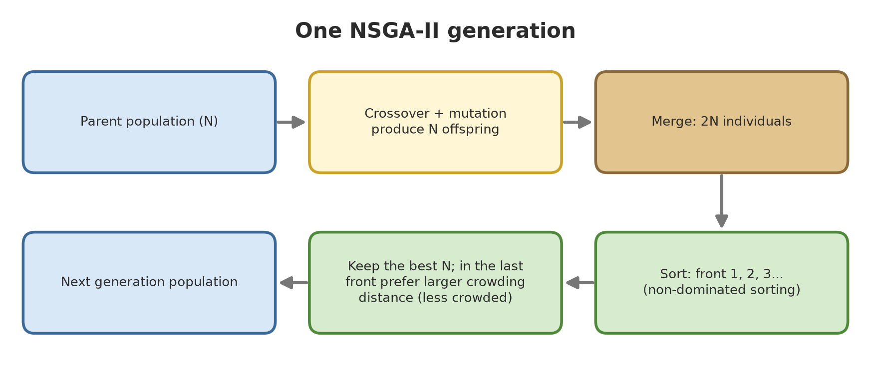
Those two ideas, non-dominated sorting (ranking into fronts 1, 2, 3…) and crowding distance, are the heart of NSGA-II (Non-dominated Sorting Genetic Algorithm II). The pymoo documentation (https://pymoo.org/algorithms/moo/nsga2.html, read 2026-10-10) explains it: individuals are chosen front by front; if only part of a front fits, the remaining places are filled by crowding distance, and the boundary points have infinite distance so they always survive.
NSGA-II with pymoo: a planting plan
pymoo is a multi-objective optimization library. You define a Problem class: the number of variables, the number of objectives, the number of constraints, and then the objective formulas in _evaluate. Two pymoo habits to remember: all objectives are minimized (profit gets a flipped sign), and constraints are written as G <= 0 meaning satisfied (the script checks this on its last line).
The problem: 20 hectares, 4 crops, two objectives (minimum cost, maximum revenue), and two constraints (available water, and at least 4 ha of rice for food). Variables from 0 to 1 are turned into hectares by dividing by their sum, so the total is always 20 ha.
04_nsga2_planting.py
# Chapter 57 - NSGA-II (pymoo): a 20 ha planting plan, two conflicting objectives (example numbers)
import numpy as np
from pymoo.algorithms.moo.nsga2 import NSGA2
from pymoo.core.problem import ElementwiseProblem
from pymoo.optimize import minimize

CROPS = ["rice", "maize", "coffee", "cocoa"]
COST = np.array([12.0, 9.0, 18.0, 16.0])        # million rupiah per ha (example)
REVENUE = np.array([22.0, 16.0, 34.0, 30.0])    # million rupiah per ha (example)
WATER = np.array([9.0, 4.0, 3.0, 3.5])          # thousand m3 per ha (example)
TOTAL_AREA, WATER_AVAILABLE, RICE_MINIMUM = 20.0, 100.0, 4.0


def area(x):
    return TOTAL_AREA * x / x.sum()              # values 0..1 become hectares that always add up to 20


class PlantingPlan(ElementwiseProblem):
    def __init__(self):
        super().__init__(n_var=4, n_obj=2, n_ieq_constr=2, xl=0.0, xu=1.0)

    def _evaluate(self, x, out, *args, **kwargs):
        ha = area(np.maximum(x, 1e-9))
        cost, revenue = COST @ ha, REVENUE @ ha
        out["F"] = [cost, -revenue]                                       # pymoo MINIMIZES; revenue gets a flipped sign
        out["G"] = [WATER @ ha - WATER_AVAILABLE,                         # G <= 0 means the constraint is satisfied
                    RICE_MINIMUM - ha[0]]


result = minimize(PlantingPlan(), NSGA2(pop_size=60), ("n_gen", 80), seed=1, verbose=False)
F = result.F
print("Number of solutions on the Pareto front:", len(F))
order = np.argsort(F[:, 0])
for name, i in [("cheapest", order[0]), ("middle", order[len(order) // 2]), ("priciest", order[-1])]:
    ha = area(result.X[i])
    print(f"{name:9s}: cost = {F[i, 0]:6.1f} | revenue = {-F[i, 1]:6.1f} | ha = "
          + ", ".join(f"{c} {h:.1f}" for c, h in zip(CROPS, ha)))
print("All solutions meet the water limit and the rice minimum:", bool((result.G <= 1e-6).all()))
Number of solutions on the Pareto front: 60
cheapest : cost = 196.4 | revenue = 352.8 | ha = rice 4.0, maize 15.5, coffee 0.5, cocoa 0.0
middle : cost = 262.8 | revenue = 485.5 | ha = rice 4.5, maize 7.8, coffee 7.6, cocoa 0.1
priciest : cost = 335.5 | revenue = 631.0 | ha = rice 4.1, maize 0.0, coffee 15.9, cocoa 0.0
All solutions meet the water limit and the rice minimum: TrueThe front has 60 solutions (the population size). Three examples: the cheapest (cost 196.4 million, revenue 352.8 million; lots of maize), the middle (cost 262.8; revenue 485.5; maize and coffee in balance), and the priciest (cost 335.5; revenue 631.0; almost all coffee). Rice stays around 4 ha because that is its minimum. All solutions meet the water and rice constraints. The manager’s job is no longer to find one answer, but to choose a point on the front that fits the capital and risk they can bear.
NSGA-II for a feed ration
The same kind of problem, in the barn: a mix of 4 feed ingredients; objectives: cost per animal per day at a minimum and daily gain at a maximum, with at least 12% protein and 15% fibre. Gain is computed by a fictitious saturating model (diminishing returns): adding protein and energy helps less and less.
05_nsga2_feed_ration.py
# Chapter 57 - NSGA-II for a cattle feed ration: cost vs daily gain (example numbers, NOT feeding advice)
import numpy as np
from pymoo.algorithms.moo.nsga2 import NSGA2
from pymoo.core.problem import ElementwiseProblem
from pymoo.optimize import minimize

INGREDIENTS = ["grass", "bran", "meal", "ground_maize"]
PRICE = np.array([800.0, 3500.0, 6500.0, 5000.0])    # rupiah per kg of feed (example)
PROTEIN = np.array([0.08, 0.12, 0.40, 0.09])         # crude protein fraction (example)
ENERGY = np.array([1.8, 2.6, 3.0, 3.4])              # Mcal per kg (example)
FIBRE = np.array([0.30, 0.12, 0.10, 0.03])           # fibre fraction (example)
DRY_MATTER_KG = 10.0                                 # allowance per animal per day


def composition(x):
    return x / x.sum()


def gain_kg_per_day(frac):
    """Fictitious model: gain rises with energy and protein, but saturates (diminishing returns)."""
    energy = (ENERGY @ frac) * DRY_MATTER_KG
    protein = (PROTEIN @ frac) * DRY_MATTER_KG
    return 1.1 * (1 - np.exp(-energy / 20)) * (1 - np.exp(-protein / 0.9))


class Ration(ElementwiseProblem):
    def __init__(self):
        super().__init__(n_var=4, n_obj=2, n_ieq_constr=2, xl=0.0, xu=1.0)

    def _evaluate(self, x, out, *args, **kwargs):
        f = composition(np.maximum(x, 1e-9))
        cost = PRICE @ f * DRY_MATTER_KG
        out["F"] = [cost, -gain_kg_per_day(f)]
        out["G"] = [0.12 - PROTEIN @ f,              # at least 12% protein
                    0.15 - FIBRE @ f]                # at least 15% fibre (rumen health)


result = minimize(Ration(), NSGA2(pop_size=60), ("n_gen", 100), seed=1, verbose=False)
F = result.F
order = np.argsort(F[:, 0])
print("Solutions on the Pareto front:", len(F))
print("cost/animal/day (Rp) | gain (kg/day) | composition")
for i in order[:: max(1, len(order) // 5)]:
    f = composition(result.X[i])
    print(f"{F[i, 0]:12,.0f} | {-F[i, 1]:9.2f} | " + ", ".join(f"{b} {p:.0%}" for b, p in zip(INGREDIENTS, f)))
Solutions on the Pareto front: 60
cost/animal/day (Rp) | gain (kg/day) | composition
15,128 | 0.50 | grass 87%, bran 0%, meal 13%, ground_maize 0%
21,847 | 0.59 | grass 76%, bran 0%, meal 24%, ground_maize 0%
28,606 | 0.66 | grass 64%, bran 0%, meal 36%, ground_maize 0%
35,788 | 0.71 | grass 51%, bran 0%, meal 49%, ground_maize 0%
42,216 | 0.75 | grass 40%, bran 1%, meal 60%, ground_maize 0%From the front: a ration at Rp15,128 per day gives 0.50 kg/day (87% grass); for 0.75 kg/day the cost climbs to Rp42,216 (60% meal). Notice the diminishing returns: going from 0.50 to 0.59 kg costs an extra Rp6,719, while going from 0.71 to 0.75 kg costs an extra Rp6,428 for only 0.04 kg. Information like this helps a farmer decide how far extra feed is still worthwhile.
NSGA-III: when there are three or more goals
With many goals (usually more than three), crowding distance is less effective. NSGA-III replaces it with reference directions: points spread evenly over the objective space, and solutions are chosen so that every direction has a representative. The pymoo documentation (https://pymoo.org/algorithms/moo/nsga3.html, read 2026-10-10) says to create them with get_reference_directions("das-dennis", number_of_objectives, n_partitions=...) and then NSGA3(pop_size=..., ref_dirs=...).
We add a third goal: wasted nitrogen (surplus protein ends up in the manure; fictitious model).
06_nsga3_three_objectives.py
# Chapter 57 - NSGA-III (pymoo): three objectives at once for the ration (cost, gain, wasted nitrogen)
import numpy as np
from pymoo.algorithms.moo.nsga3 import NSGA3
from pymoo.core.problem import ElementwiseProblem
from pymoo.optimize import minimize
from pymoo.util.ref_dirs import get_reference_directions

PRICE = np.array([800.0, 3500.0, 6500.0, 5000.0])    # rupiah per kg (example)
PROTEIN = np.array([0.08, 0.12, 0.40, 0.09])
ENERGY = np.array([1.8, 2.6, 3.0, 3.4])
FIBRE = np.array([0.30, 0.12, 0.10, 0.03])
KG = 10.0


class RationThreeObjectives(ElementwiseProblem):
    def __init__(self):
        super().__init__(n_var=4, n_obj=3, n_ieq_constr=2, xl=0.0, xu=1.0)

    def _evaluate(self, x, out, *args, **kwargs):
        f = np.maximum(x, 1e-9)
        f = f / f.sum()
        energy, protein = (ENERGY @ f) * KG, (PROTEIN @ f) * KG
        gain = 1.1 * (1 - np.exp(-energy / 20)) * (1 - np.exp(-protein / 0.9))
        cost = PRICE @ f * KG
        nitrogen = max(0.0, protein - 0.16 * gain * 2.0)         # surplus protein leaves in the manure (fictitious model)
        out["F"] = [cost / 1000, -gain * 10, nitrogen]           # all minimized; scaled to be comparable
        out["G"] = [0.12 - PROTEIN @ f, 0.15 - FIBRE @ f]


# Reference points spread evenly over the objective triangle; their number (n_partitions=8, 3 objectives) = C(10,2) = 45
ref_dirs = get_reference_directions("das-dennis", 3, n_partitions=8)
print("Number of reference directions:", len(ref_dirs))
result = minimize(RationThreeObjectives(), NSGA3(pop_size=len(ref_dirs), ref_dirs=ref_dirs),
                  ("n_gen", 150), seed=1, verbose=False)
F = result.F
print("Final solutions:", len(F))
print("Range of each objective (min - max):")
for name, k in [("cost (thousand Rp)", 0), ("-gain x10", 1), ("wasted nitrogen", 2)]:
    print(f"  {name:20s} {F[:, k].min():8.2f} - {F[:, k].max():8.2f}")
Number of reference directions: 45
Final solutions: 21
Range of each objective (min - max):
cost (thousand Rp) 15.15 - 49.97
-gain x10 -7.88 - -5.05
wasted nitrogen 1.02 - 2.90With 3 objectives and n_partitions=8, 45 reference directions are formed (the count is C(10,2) = 45). Of the 45 individuals, 21 remain as the final non-dominated solutions. The range of each objective shows how wide the choice is: cost 15.15 to 49.97 thousand rupiah, gain (times 10) 5.05 to 7.88, wasted nitrogen 1.02 to 2.90.
PSO and simulated annealing
Two other methods, both for a single objective, with no derivatives needed:
- PSO (particle swarm optimization): a swarm of particles flies over the search map, each pulled toward its own best record and the swarm’s best record, like a flock of birds looking for food.
- Simulated annealing: a random walk toward better points, but with a chance of accepting a worse step that shrinks as the “temperature” falls, like metal cooled slowly. This helps it escape local traps.
The problem: place a fertilizer depot so the total distance to 8 gardens is minimal (example coordinates).
07_pso_sa.py
# Chapter 57 - PSO (particle swarm) and simulated annealing: place a fertilizer depot to minimize distance to 8 gardens
import math
import random

import numpy as np

random.seed(1)
rng = np.random.default_rng(1)
GARDENS = np.array([[1, 1], [2, 8], [4, 5], [6, 2], [7, 7], [8, 4], [9, 9], [3, 3]], dtype=float)   # km (example)


def total_distance(point):
    return float(np.sqrt(((GARDENS - point) ** 2).sum(axis=1)).sum())


# --- PSO: 20 particles fly over the map; each is pulled toward its own record and the swarm's record
position = rng.uniform(0, 10, (20, 2))
velocity = np.zeros((20, 2))
personal_best = position.copy()
personal_value = np.array([total_distance(p) for p in position])
swarm_best = personal_best[personal_value.argmin()].copy()
for _ in range(60):
    r1, r2 = rng.random((20, 2)), rng.random((20, 2))
    velocity = 0.7 * velocity + 1.5 * r1 * (personal_best - position) + 1.5 * r2 * (swarm_best - position)
    position = np.clip(position + velocity, 0, 10)
    value = np.array([total_distance(p) for p in position])
    improved = value < personal_value
    personal_best[improved], personal_value[improved] = position[improved], value[improved]
    swarm_best = personal_best[personal_value.argmin()].copy()
print("PSO               : point =", swarm_best.round(2).tolist(), "| total distance =", round(total_distance(swarm_best), 3))

# --- Simulated annealing: may accept worse steps, especially when the "temperature" is high
point = np.array([random.uniform(0, 10), random.uniform(0, 10)])
best, best_value = point.copy(), total_distance(point)
temperature = 5.0
for step in range(3000):
    candidate = np.clip(point + np.array([random.gauss(0, 0.5), random.gauss(0, 0.5)]), 0, 10)
    difference = total_distance(candidate) - total_distance(point)
    if difference < 0 or random.random() < math.exp(-difference / temperature):    # chance to accept a bad step
        point = candidate
        if total_distance(point) < best_value:
            best, best_value = point.copy(), total_distance(point)
    temperature *= 0.998                                              # cooled slowly
print("Simulated annealing: point =", best.round(2).tolist(), "| total distance =", round(best_value, 3))

# Comparison: brute-force search on a 0.05 km grid
grid = [(x, y) for x in np.arange(0, 10.01, 0.05) for y in np.arange(0, 10.01, 0.05)]
best_grid = min(grid, key=lambda p: total_distance(np.array(p)))
print("Grid comparison    : point =", [round(float(v), 2) for v in best_grid], "| total distance =", round(total_distance(np.array(best_grid)), 3))
PSO : point = [4.57, 4.74] | total distance = 28.356
Simulated annealing: point = [4.56, 4.74] | total distance = 28.356
Grid comparison : point = [4.55, 4.75] | total distance = 28.356All three agree on a total distance of 28.356 km around (4.56, 4.74). PSO and simulated annealing find practically the same point as a brute-force search on a 0.05 km grid. A grid comparison is only possible in a 2-dimensional problem; with dozens of variables, that is exactly where these methods earn their keep.
Bayesian optimization and Optuna
Training a model is expensive, so blindly trying hundreds of hyperparameter combinations is wasteful. Bayesian optimization builds a model from earlier trials to guess which combination is worth trying next. Optuna is a popular library for this. Its default sampler is TPESampler (Tree-structured Parzen Estimator; the Optuna documentation, read 2026-10-10, recommends 100-1000 trials, and we use only 25-40 to keep it fast).
The script uses the land data from Chapter 54 with block cross-validation. First one objective (accuracy), then two objectives (accuracy vs model size; “size” = number of trees x depth, a stable stand-in for prediction time):
08_optuna.py
# Chapter 57 - Optuna: finding hyperparameters with Bayesian optimization (TPE), one and two objectives
import optuna
from sklearn.ensemble import RandomForestClassifier
from sklearn.model_selection import GroupKFold, cross_val_score

from make_data import FEATURES, make_land   # helper module: a copy from Chapter 54, in the same folder

optuna.logging.set_verbosity(optuna.logging.WARNING)
df = make_land()
X, y, groups = df[FEATURES], df["land_class"], df["block"]


def accuracy(trees, depth, max_features):
    model = RandomForestClassifier(n_estimators=trees, max_depth=depth, max_features=max_features,
                                   random_state=42, n_jobs=1)
    return cross_val_score(model, X, y, groups=groups, cv=GroupKFold(n_splits=4)).mean()


# 1) One objective: accuracy as high as possible (block cross-validation from Chapter 54)
def single_objective(trial):
    return accuracy(trial.suggest_int("n_estimators", 20, 200, step=20),
                    trial.suggest_int("max_depth", 2, 12),
                    trial.suggest_float("max_features", 0.25, 1.0))


study = optuna.create_study(direction="maximize", sampler=optuna.samplers.TPESampler(seed=42))
study.optimize(single_objective, n_trials=25)
print("One objective  - best accuracy:", round(study.best_value, 3))
print("                 hyperparameters:", {k: (round(v, 2) if isinstance(v, float) else v) for k, v in study.best_params.items()})


# 2) Two objectives: accuracy (max) vs model size (min). Size = trees x depth, a stable proxy for prediction time
def two_objectives(trial):
    trees = trial.suggest_int("n_estimators", 20, 200, step=20)
    depth = trial.suggest_int("max_depth", 2, 12)
    return accuracy(trees, depth, 0.75), trees * depth


study2 = optuna.create_study(directions=["maximize", "minimize"], sampler=optuna.samplers.NSGAIISampler(seed=42))
study2.optimize(two_objectives, n_trials=40)
front = sorted(study2.best_trials, key=lambda t: t.values[1])
print("\nTwo objectives - number of Pareto solutions:", len(front))
print("size (trees x depth) | accuracy")
for t in front:
    print(f"{t.values[1]:14.0f}       | {t.values[0]:.3f}")
One objective - best accuracy: 0.889
hyperparameters: {'n_estimators': 200, 'max_depth': 12, 'max_features': 0.55}
Two objectives - number of Pareto solutions: 6
size (trees x depth) | accuracy
80 | 0.868
100 | 0.876
280 | 0.881
280 | 0.881
540 | 0.885
1280 | 0.885- One objective: best accuracy 0.889 with 200 trees, depth 12, and 55% of features per split.
- Two objectives: 6 Pareto solutions. A model of size 80 (for example 20 trees of depth 4) already reaches 0.868; a model 16 times bigger (1280) only rises to 0.885. Two objectives show that the last bit of accuracy is very expensive, information lost if we only chase accuracy.
- The two rows with size 280 have the same value: two different combinations that give similar results.
The same can be done for YOLO hyperparameters (mAP accuracy vs inference speed): trial.suggest_* and then train YOLO inside the objective function. We do not run it in the book because one trial takes 2 to 3 minutes on a GPU (Chapter 56), so dozens of trials would take too long for an automatic build. The code pattern is the same as in the script above.
Running Project A3: choosing one ration and proving the value of NSGA-II
Two questions remain: (1) how do we pick one point from the front? (2) is NSGA-II really better than random trials with the same number of evaluations? The answer to (2) uses the hypervolume: the area of objective space “dominated” by the front relative to a worst-case reference point (larger is better).
09_project_pick_solution.py
# Chapter 57 - Project A3: pick one ration from the Pareto front, and prove NSGA-II beats random trial and error
import numpy as np
from pymoo.algorithms.moo.nsga2 import NSGA2
from pymoo.core.problem import ElementwiseProblem
from pymoo.indicators.hv import HV
from pymoo.mcdm.pseudo_weights import PseudoWeights
from pymoo.optimize import minimize

INGREDIENTS = ["grass", "bran", "meal", "ground_maize"]
PRICE = np.array([800.0, 3500.0, 6500.0, 5000.0])
PROTEIN = np.array([0.08, 0.12, 0.40, 0.09])
ENERGY = np.array([1.8, 2.6, 3.0, 3.4])
FIBRE = np.array([0.30, 0.12, 0.10, 0.03])
KG = 10.0


def compute(x):
    f = np.maximum(x, 1e-9)
    f = f / f.sum()
    gain = 1.1 * (1 - np.exp(-(ENERGY @ f) * KG / 20)) * (1 - np.exp(-(PROTEIN @ f) * KG / 0.9))
    return f, PRICE @ f * KG, gain, [0.12 - PROTEIN @ f, 0.15 - FIBRE @ f]


class Ration(ElementwiseProblem):
    def __init__(self):
        super().__init__(n_var=4, n_obj=2, n_ieq_constr=2, xl=0.0, xu=1.0)

    def _evaluate(self, x, out, *args, **kwargs):
        _, cost, gain, g = compute(x)
        out["F"], out["G"] = [cost / 1000, -gain], g             # cost in thousand rupiah


problem = Ration()
result = minimize(problem, NSGA2(pop_size=60), ("n_gen", 100), seed=1, verbose=False)   # 60 x 100 = 6,000 evaluations

# Comparison: 6,000 random rations that meet the requirements
rng = np.random.default_rng(1)
random_set = []
for _ in range(6000):
    x = rng.random(4)
    _, cost, gain, g = compute(x)
    if max(g) <= 0:
        random_set.append([cost / 1000, -gain])
random_set = np.array(random_set)
reference = np.array([60.0, 0.0])                                # hypervolume reference point: cost 60 thousand, gain 0
hv = HV(ref_point=reference)
print("Random rations that meet the requirements:", len(random_set), "of 6000")
print("Hypervolume NSGA-II :", round(float(hv(result.F)), 2))
print("Hypervolume random  :", round(float(hv(random_set)), 2), "(larger = better front)")

# Picking one solution: the decision maker's preference weights (60% cost, 40% gain)
i = PseudoWeights(np.array([0.6, 0.4])).do(result.F)
f, cost, gain, _ = compute(result.X[i])
print("\nChosen ration (preference 60% saving cost, 40% gain):")
print("  composition:", ", ".join(f"{b} {p:.0%}" for b, p in zip(INGREDIENTS, f)))
print(f"  cost {cost:,.0f} Rp/animal/day | gain {gain:.2f} kg/day")
print("  Note: fictitious model; real rations are formulated with a livestock nutritionist.")
Random rations that meet the requirements: 1677 of 6000
Hypervolume NSGA-II : 31.32
Hypervolume random : 29.01 (larger = better front)
Chosen ration (preference 60% saving cost, 40% gain):
composition: grass 68%, bran 0%, meal 32%, ground_maize 0%
cost 26,454 Rp/animal/day | gain 0.64 kg/day
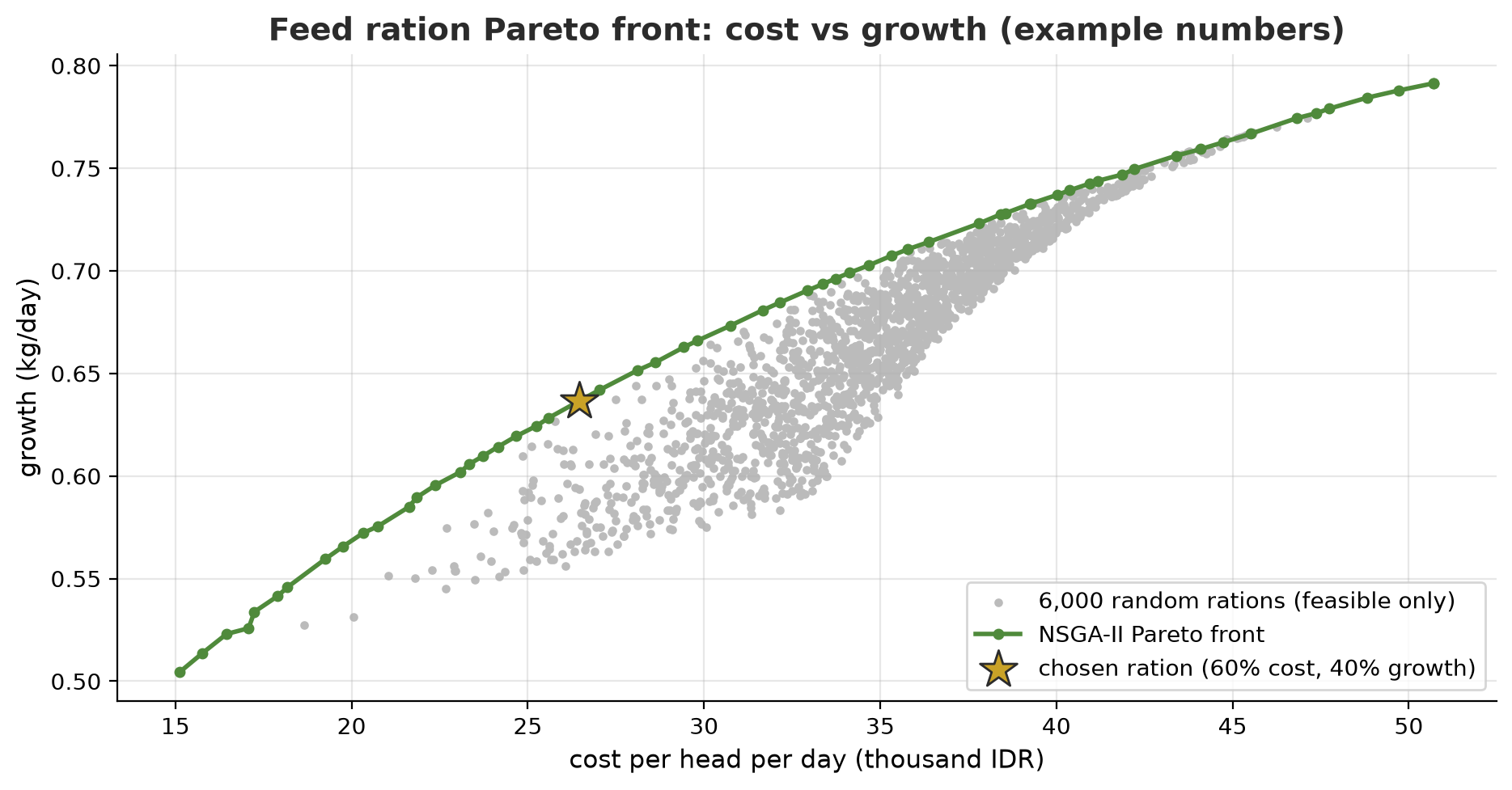
Note: fictitious model; real rations are formulated with a livestock nutritionist.- Of 6,000 random rations, only 1,677 meet the protein and fibre requirements; the rest break them. The random hypervolume is 29.01 and NSGA-II’s is 31.32 with the same number of evaluations (60 x 100 = 6,000): NSGA-II is better, because it concentrates the search on promising regions.
- PseudoWeights takes the decision maker’s preference weights (here 60% for saving cost, 40% for gain) and picks the solution on the front that fits best: 68% grass + 32% meal, cost Rp26,454 per animal per day, gain 0.64 kg/day (the star in the figure). The human decision maker still sets the weights.
The results of this project carry on to Chapter 59, where the planting plan and the ration become part of an agricultural information system.
Exercises
- In
01_ga_manual.py, change the mutation probability from 0.05 to 0.0 and to 0.3. How does the final fitness change, and why? - In
04_nsga2_planting.py, raiseRICE_MINIMUMto 10 ha. How does the front shift? Are there still solutions that meet the water limit? - In
08_optuna.py, changen_trialsin the one-objective study to 10 and 60. Does the best accuracy always go up? - Challenge: add a third objective to
04_nsga2_planting.py: total water need (minimized), turn the water constraint into an objective, and then run NSGA-III as in script 06.
Chapter Summary
- Genetic algorithm: population, selection, crossover, mutation, elitism; the answer is good but not guaranteed optimal (GA 342.0 vs exact 345.0).
- Dominance and the Pareto front: the set of best compromises when goals conflict.
- NSGA-II: sort into fronts (non-dominated sorting) and keep variety with crowding distance; NSGA-III: reference directions for three or more objectives.
- pymoo minimizes all objectives and uses
G <= 0for constraints; DEAP uses tuple fitness and weights. - PSO, simulated annealing, and Optuna (TPE) for a single objective; Optuna also supports multi-objective.
- Picking one solution from the front is a human decision (preferences, pseudo-weights), and the hypervolume proves the quality of the front.
Next, in Chapter 58: the model is smart and the choices are optimal, but can we explain and trust it? Chapter 58 covers SHAP, MLflow, drift monitoring, and responsible AI.