Chapter 54 — Classical Machine Learning: Trees, Forests, and Boosting
Series A3 — Machine Learning for Natural Resources
All scripts for this chapter are in the kode/ch54/ folder. On the web version, you can also download them all at once (zip).
In Series I3 you modeled data with regression: you chose the shape of the formula. In machine learning (ML), the direction is reversed: you give examples (data with answers), and the computer finds the rules by itself. Picture a forest ranger who has looked at land plots on satellite photos for years. In the end he knows by heart: “dark green, tall, steep: forest; light green, flat, near water: rice field.” ML does something similar, only from thousands of examples in a matter of seconds.
This chapter uses classical ML: models that work on tables of numbers and are very dependable for field data. Chapter 55 covers neural networks (deep learning) and GPUs.
All the data in this chapter is fictitious, made by a script (make_data.py): 1,200 land plots on a made-up 1,000 x 1,000 meter map, with the features NDVI (vegetation greenness index), elevation, slope, and rainfall. The accuracy numbers in the book are example numbers, not real ability in an actual forest.
Data: land plots with a class
Each plot has four features (clues for guessing) and one label (the answer: forest, plantation, rice_field, or settlement). The fictitious map is built from 40 land “patches”, so neighboring plots tend to share a class, as in the real world. This matters in the spatial validation section later.
Decision tree
A decision tree is a chain of yes/no questions, like a guessing game: “Is NDVI above 0.3? Is the slope above 13? …” until it arrives at an answer. Its big advantage: the rules are readable by humans.
01_decision_tree.py
# Chapter 54 - Decision tree: "if-then" rules learned from data
from sklearn.model_selection import train_test_split
from sklearn.tree import DecisionTreeClassifier, export_text

from make_data import FEATURES, make_land

df = make_land()
print("Data shape:", df.shape)
print(df["land_class"].value_counts().sort_index().to_string())

X_train, X_test, y_train, y_test = train_test_split(
    df[FEATURES], df["land_class"], test_size=0.25, random_state=42, stratify=df["land_class"])

tree = DecisionTreeClassifier(max_depth=3, random_state=42)
tree.fit(X_train, y_train)
print("\nRules learned:")
print(export_text(tree, feature_names=FEATURES, decimals=3))
print("Training accuracy:", round(tree.score(X_train, y_train), 3))
print("Test accuracy    :", round(tree.score(X_test, y_test), 3))
Data shape: (1200, 8)
land_class
forest 198
plantation 146
rice_field 326
settlement 530
Rules learned:
|--- ndvi <= 0.313
| |--- ndvi <= 0.229
| | |--- elevation_m <= 306.000
| | | |--- class: settlement
| | |--- elevation_m > 306.000
| | | |--- class: plantation
| |--- ndvi > 0.229
| | |--- elevation_m <= 155.500
| | | |--- class: settlement
| | |--- elevation_m > 155.500
| | | |--- class: rice_field
|--- ndvi > 0.313
| |--- elevation_m <= 235.500
| | |--- elevation_m <= 171.500
| | | |--- class: rice_field
| | |--- elevation_m > 171.500
| | | |--- class: plantation
| |--- elevation_m > 235.500
| | |--- slope_degrees <= 13.350
| | | |--- class: plantation
| | |--- slope_degrees > 13.350
| | | |--- class: forest
Training accuracy: 0.88
Test accuracy : 0.807- The data is split in two: 75% for training (learning), 25% for testing (an exam with questions the model has never seen).
stratifykeeps the class proportions the same in both parts.random_state=42locks the shuffling so the result is the same every run. max_depth=3limits the tree to three levels of questions.- Read the tree from the top. The first question is
ndvi <= 0.313. On the low-NDVI side, a very dull plot (ndvi <= 0.229) with low elevation ends assettlement, and the same plot at higher elevation ends asplantation. On the high-NDVI side, a plot above 235.5 m with a steep slope (slope_degrees > 13.350) ends asforest. - The tree is also allowed to be wrong: some leaves mix classes, and the tree simply names the most common one.
- Training accuracy is 0.88 and test accuracy is 0.807. The gap of 0.073 is already a small hint that even this little tree fits the training plots a bit better than new ones.
Overfitting: when the model memorizes
A student who memorizes the answer key scores 100 on the practice sheet but flops on an exam with new questions. That is overfitting. We can see it by letting the tree grow deeper:
02_overfitting.py
# Chapter 54 - Overfitting: a tree that is too deep memorizes the training data
from sklearn.model_selection import train_test_split
from sklearn.tree import DecisionTreeClassifier

from make_data import FEATURES, make_land

df = make_land()
X_train, X_test, y_train, y_test = train_test_split(
    df[FEATURES], df["land_class"], test_size=0.25, random_state=42, stratify=df["land_class"])

print("depth | train accuracy | test accuracy | gap")
for depth in [1, 2, 3, 5, 8, 12, None]:
    tree = DecisionTreeClassifier(max_depth=depth, random_state=42).fit(X_train, y_train)
    acc_train = tree.score(X_train, y_train)
    acc_test = tree.score(X_test, y_test)
    print(f"{str(depth):>5} | {acc_train:14.3f} | {acc_test:13.3f} | {acc_train - acc_test:7.3f}")
depth | train accuracy | test accuracy | gap
1 | 0.652 | 0.647 | 0.006
2 | 0.811 | 0.810 | 0.001
3 | 0.880 | 0.807 | 0.073
5 | 0.927 | 0.857 | 0.070
8 | 0.973 | 0.833 | 0.140
12 | 1.000 | 0.820 | 0.180
None | 1.000 | 0.820 | 0.180Training accuracy keeps climbing until it reaches 1.000 (a tree with no limit memorizes every plot), while test accuracy stops improving around depth 5 (0.857) and then drops to 0.820. The gap widens from 0.006 at depth 1 to 0.180.
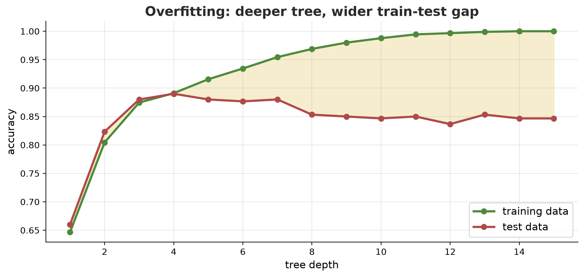
High accuracy on the training data proves nothing. What matters is the score on data the model has never seen. Never report a training score as the model’s ability.
Random forest: many trees, one vote
One tree is easily wrong. A random forest builds hundreds of trees, each trained on a randomly resampled copy of the data and choosing from only some of the features at random. The final answer is taken by voting. Like a village meeting: one person can be mistaken, but the majority is usually wiser.
03_random_forest.py
# Chapter 54 - Random forest: many trees "vote", plus feature importance
from sklearn.ensemble import RandomForestClassifier
from sklearn.metrics import classification_report
from sklearn.model_selection import train_test_split
from sklearn.tree import DecisionTreeClassifier

from make_data import FEATURES, make_land

df = make_land()
X_train, X_test, y_train, y_test = train_test_split(
    df[FEATURES], df["land_class"], test_size=0.25, random_state=42, stratify=df["land_class"])

single = DecisionTreeClassifier(random_state=42).fit(X_train, y_train)
forest = RandomForestClassifier(n_estimators=200, oob_score=True, random_state=42, n_jobs=1)
forest.fit(X_train, y_train)

print("One tree (no limit)       - test accuracy:", round(single.score(X_test, y_test), 3))
print("Random forest, 200 trees  - test accuracy:", round(forest.score(X_test, y_test), 3))
print("OOB score (no test data)  :", round(forest.oob_score_, 3))

print("\nFeature importance (sum = 1):")
for name, value in sorted(zip(FEATURES, forest.feature_importances_), key=lambda p: -p[1]):
    print(f"  {name:20s} {value:.3f}")

print("\nPer-class report:")
print(classification_report(y_test, forest.predict(X_test), digits=2))
One tree (no limit) - test accuracy: 0.82
Random forest, 200 trees - test accuracy: 0.863
OOB score (no test data) : 0.898
Feature importance (sum = 1):
ndvi 0.457
elevation_m 0.289
slope_degrees 0.188
rainfall_mm 0.065
Per-class report:
precision recall f1-score support
forest 0.96 0.92 0.94 50
plantation 0.70 0.78 0.74 36
rice_field 0.78 0.79 0.79 82
settlement 0.93 0.91 0.92 132
accuracy 0.86 300
macro avg 0.84 0.85 0.85 300
weighted avg 0.87 0.86 0.86 300- One tree with no limit: 0.82. A random forest of 200 trees: 0.863. Combining many trees dampens overfitting.
- The OOB score (out-of-bag, 0.898) is a free exam: each tree does not see about a third of the data, and exactly that data is used to grade it. The result is close to the test accuracy, so even without test data we have an honest estimate. (It is a little higher than 0.863 here; with only 300 test plots, a gap like this is ordinary noise.)
- Feature importance:
ndvimatters most (0.457), rainfall least (0.065). They all add up to 1. This is the average of how much each feature reduces impurity across all the trees. - Per-class report:
precision(of the plots guessed as rice field, how many were right) andrecall(of all the real rice fields, how many were caught). Theplantationclass is the hardest (f1 0.74), because it resembles rice field and forest.
The built-in feature importance of a random forest can be misleading when features are correlated (NDVI and elevation are often related). Chapter 58 teaches a fairer way: SHAP and permutation importance.
Gradient boosting: learning from mistakes
A random forest builds trees side by side (independent). Gradient boosting builds trees one after another: the second tree is trained specifically to fix the mistakes of the first, the third fixes what is left over from the first two, and so on. Like a farmer who corrects last season’s mistakes each season.
Three popular implementations: GradientBoostingClassifier (scikit-learn), XGBoost, and LightGBM. All three are used with the same .fit() and .score() pattern.
04_boosting.py
# Chapter 54 - Gradient boosting: small trees added one by one to fix the errors
from lightgbm import LGBMClassifier
from sklearn.ensemble import GradientBoostingClassifier
from sklearn.model_selection import train_test_split
from sklearn.preprocessing import LabelEncoder
from xgboost import XGBClassifier

from make_data import FEATURES, make_land

df = make_land()
encoder = LabelEncoder().fit(df["land_class"])    # XGBoost needs classes as numbers 0,1,2,3
y = encoder.transform(df["land_class"])
X_train, X_test, y_train, y_test = train_test_split(
    df[FEATURES], y, test_size=0.25, random_state=42, stratify=y)

models = {
    "sklearn GradientBoosting": GradientBoostingClassifier(n_estimators=100, max_depth=3, random_state=42),
    "XGBoost": XGBClassifier(n_estimators=100, max_depth=3, learning_rate=0.1, random_state=42, n_jobs=1),
    "LightGBM": LGBMClassifier(n_estimators=100, max_depth=3, learning_rate=0.1, random_state=42,
                               n_jobs=1, verbose=-1),
}
for name, m in models.items():
    m.fit(X_train, y_train)
    print(f"{name:26s} test accuracy = {m.score(X_test, y_test):.3f}")
print("Class order (number -> name):", list(encoder.classes_))
sklearn GradientBoosting test accuracy = 0.863
XGBoost test accuracy = 0.867
LightGBM test accuracy = 0.860
Class order (number -> name): ['forest', 'plantation', 'rice_field', 'settlement']All three are nearly the same (0.860 to 0.867) on this small data. XGBoost and LightGBM shine when the data is large (tens of thousands of rows and up) because they are very fast and have many extra features (handling missing values, early stopping). Note: XGBoost demands labels as numbers, so the classes are converted first by LabelEncoder, which numbers them in alphabetical order (the last line of the output shows the order).
SVM and k-means
An SVM (support vector machine) looks for the best boundary between classes. k-means is grouping without labels: it just gathers similar plots into k clusters. Both are sensitive to the scale of the numbers: elevation (hundreds) would “beat” NDVI (below 1) unless we put them on the same scale with StandardScaler.
05_svm_kmeans.py
# Chapter 54 - SVM (with scaling) and k-means (no labels)
from sklearn.cluster import KMeans
from sklearn.metrics import adjusted_rand_score
from sklearn.model_selection import train_test_split
from sklearn.pipeline import make_pipeline
from sklearn.preprocessing import StandardScaler
from sklearn.svm import SVC

from make_data import FEATURES, make_land

df = make_land()
X_train, X_test, y_train, y_test = train_test_split(
    df[FEATURES], df["land_class"], test_size=0.25, random_state=42, stratify=df["land_class"])

unscaled = SVC(kernel="rbf").fit(X_train, y_train)
scaled = make_pipeline(StandardScaler(), SVC(kernel="rbf")).fit(X_train, y_train)
print("SVM without scaling - test accuracy:", round(unscaled.score(X_test, y_test), 3))
print("SVM with scaling    - test accuracy:", round(scaled.score(X_test, y_test), 3))

# k-means is NOT given labels; it only groups similar plots together
X_scaled = StandardScaler().fit_transform(df[FEATURES])
km = KMeans(n_clusters=4, n_init=10, random_state=42).fit(X_scaled)
df["cluster"] = km.labels_
print("\nCross-table of k-means clusters (rows) x true classes (columns):")
print(df.groupby(["cluster", "land_class"]).size().unstack(fill_value=0).to_string())
print("Adjusted Rand Index (1 = perfect match):", round(adjusted_rand_score(df["land_class"], df["cluster"]), 3))
SVM without scaling - test accuracy: 0.613
SVM with scaling - test accuracy: 0.897
Cross-table of k-means clusters (rows) x true classes (columns):
land_class forest plantation rice_field settlement
cluster
0 0 1 94 215
1 195 18 0 0
2 0 3 154 313
3 3 124 78 2
Adjusted Rand Index (1 = perfect match): 0.367- SVM without scaling reaches only 0.613, with scaling 0.897. One extra line changes everything.
- k-means never saw the labels. Cluster 1 is almost pure
forest(195 of its 213 plots), butrice_fieldandsettlementare mixed together in clusters 0 and 2, and cluster 3 mixesplantation(124) withrice_field(78). The Adjusted Rand Index of 0.367 (1 = perfect match) shows that unlabeled clusters are no replacement for labeled classification, but they are useful for early exploration.
Trees, random forests, and boosting do not need scaling because they only compare “bigger or smaller than a threshold”. SVM, k-means, regression, and neural networks do need it.
Cross-validation
A single train/test split depends on the luck of the split. Cross-validation divides the data into k folds, then takes turns using one fold for testing and the rest for training.
06_cross_validation.py
# Chapter 54 - Cross-validation: testing the model many times on different pieces of data
from sklearn.ensemble import RandomForestClassifier
from sklearn.model_selection import KFold, cross_val_score

from make_data import FEATURES, make_land

df = make_land()
X, y = df[FEATURES], df["land_class"]
model = RandomForestClassifier(n_estimators=100, random_state=42, n_jobs=1)

folds = KFold(n_splits=5, shuffle=True, random_state=42)
scores = cross_val_score(model, X, y, cv=folds, scoring="accuracy")
print("Accuracy of each fold:", scores.round(3))
print(f"Mean = {scores.mean():.3f}   standard deviation = {scores.std():.3f}")
Accuracy of each fold: [0.879 0.883 0.888 0.888 0.912]
Mean = 0.890 standard deviation = 0.012Five folds, five scores (0.879 to 0.912), mean 0.890. The standard deviation of 0.012 gives a feel for how stable the model is. Reporting “0.890 ± 0.012” is far more honest than a single number.
Spatial data: random folds cheat
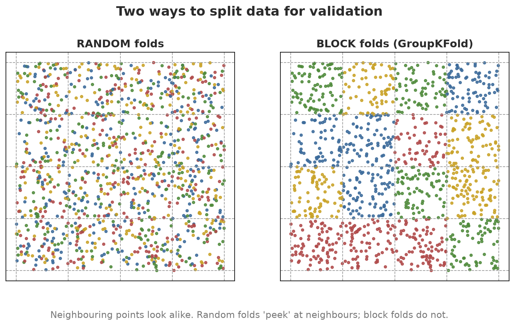
The first law of geography: everything is related to everything else, but near things are more related than distant things. Because neighboring plots look alike, random folds put twin neighbors in both the training and the test fold: the model “peeks” at its neighbors. The score is too good to rely on in a new area.
The remedy: spatial cross-validation. Divide the map into blocks (grid cells), then make sure a whole block stays in the same fold. In scikit-learn, use GroupKFold with the block column as groups.
07_spatial_cv.py
# Chapter 54 - Spatial cross-validation: folds by geographic block (GroupKFold on grid cells)
from sklearn.ensemble import RandomForestClassifier
from sklearn.model_selection import GroupKFold, KFold, cross_val_score

from make_data import FEATURES, make_land

df = make_land()
y = df["land_class"]
model = RandomForestClassifier(n_estimators=100, random_state=42, n_jobs=1)
print("Number of blocks (250 m grid cells):", df["block"].nunique())

for title, columns in [("image features only", FEATURES), ("features + x,y coordinates", FEATURES + ["x", "y"])]:
    rand = cross_val_score(model, df[columns], y, cv=KFold(5, shuffle=True, random_state=42))
    block = cross_val_score(model, df[columns], y, groups=df["block"], cv=GroupKFold(n_splits=4))
    print(f"\n{title}")
    print(f"  RANDOM folds: accuracy = {rand.mean():.3f}")
    print(f"  BLOCK folds : accuracy = {block.mean():.3f}")
Number of blocks (250 m grid cells): 16
image features only
RANDOM folds: accuracy = 0.890
BLOCK folds : accuracy = 0.885
features + x,y coordinates
RANDOM folds: accuracy = 0.922
BLOCK folds : accuracy = 0.876- With image features only, the gap between random and block is small (0.890 vs 0.885), because the relation from features to class is about the same across the whole map.
- Once the x, y coordinates become features too, the random folds jump to 0.922 (the model memorizes “at this spot, the class is so-and-so”) but the block folds fall to 0.876, even below the model without coordinates. That is real spatial leakage.
If the model will be used in another area or at another time, test it that way: block folds for areas, per-year folds for time. The block size should be larger than the distance over which plots resemble each other. Blocks that are too small still leak.
When is classical ML better than deep learning?
| Situation | Usually the right choice |
|---|---|
| Tabular data (number columns), thousands to hundreds of thousands of rows | Classical ML (random forest, boosting) |
| Little data, limited budget, no GPU | Classical ML |
| You need an explanation (“why is this plot a rice field?”) | Classical ML (trees are easy to explain) |
| Raw image data, audio, long text | Deep learning (Chapters 55 and 56) |
| Millions of examples and very complex patterns | Deep learning |
Rule of thumb: for tabular data, start with a random forest or LightGBM. Only when it proves lacking, consider a heavier model. The experience of many practitioners is that tree-based models are often hard to beat on tabular data.
Running Project A3: land cover and harvest
We put it all together: (1) land-cover classification with a random forest scored with block folds, (2) rice harvest prediction (example numbers, not cultivation advice) with a random forest compared to linear regression.
08_project_rf_land_harvest.py
# Chapter 54 - Project A3: random forest for land cover (classification) and harvest (regression)
import numpy as np
from sklearn.ensemble import RandomForestClassifier, RandomForestRegressor
from sklearn.linear_model import LinearRegression
from sklearn.metrics import confusion_matrix
from sklearn.model_selection import GroupKFold, cross_val_predict, cross_val_score

from make_data import FEATURES, make_land

df = make_land()
folds = GroupKFold(n_splits=4)

# 1) Land-cover classification, scored with BLOCK folds
rf = RandomForestClassifier(n_estimators=200, random_state=42, n_jobs=1)
predicted = cross_val_predict(rf, df[FEATURES], df["land_class"], groups=df["block"], cv=folds)
names = sorted(df["land_class"].unique())
print("Confusion matrix (rows = actual, columns = predicted):", names)
print(confusion_matrix(df["land_class"], predicted, labels=names))
print("Accuracy (block):", round((predicted == df["land_class"]).mean(), 3))

# 2) Rice harvest regression (example numbers): the relation is made curved so a linear model struggles
rng = np.random.default_rng(7)
rice = df[df["land_class"] == "rice_field"].copy()
rice["harvest_kg_ha"] = (4000 + 5000 * np.sin(np.pi * rice["ndvi"].clip(0, 1))
                         + 0.8 * (rice["rainfall_mm"] - 2200) + rng.normal(0, 250, len(rice))).round(0)
columns = ["ndvi", "rainfall_mm", "elevation_m"]
for model_name, model in [("Linear regression", LinearRegression()),
                          ("Random forest    ", RandomForestRegressor(n_estimators=200, random_state=42, n_jobs=1))]:
    r2 = cross_val_score(model, rice[columns], rice["harvest_kg_ha"], groups=rice["block"],
                         cv=GroupKFold(n_splits=4), scoring="r2")
    print(f"{model_name}: R2 block folds = {r2.mean():.3f}")
print("Number of rice plots:", len(rice))
Confusion matrix (rows = actual, columns = predicted): ['forest', 'plantation', 'rice_field', 'settlement']
[[186 12 0 0]
[ 12 115 18 1]
[ 0 15 270 41]
[ 0 0 40 490]]
Accuracy (block): 0.884
Linear regression: R2 block folds = 0.130
Random forest : R2 block folds = 0.758
Number of rice plots: 326- Confusion matrix: the diagonal holds the correct guesses. The most frequent mistakes: 41
rice_fieldplots guessed assettlementand 40 the other way around; 18plantationplots guessed asrice_field. The accuracy with block folds is 0.884. The error pattern tells you which classes need extra features (for example imagery from another season). - Harvest: linear regression gets only R² 0.130 (1 = perfect), the random forest 0.758. In this data the relation from NDVI to harvest is curved (rises, then falls), and a linear model cannot imitate that. Because we used blocks for validation, the 0.758 is more trustworthy for a new area.
- There are 326 rice plots in this fictitious data.
The models and knowledge from this chapter are used again in Chapter 58 (SHAP explanations, MLflow tracking) and Chapter 59 (from satellite imagery to a map).
Exercises
- Change
max_depthin01_decision_tree.pyto 2 and 4. How do the rules and the test accuracy change? - In
03_random_forest.py, replacen_estimators=200with 10, 50, and 500. Does the OOB score keep rising? How many trees are “enough”? - In
05_svm_kmeans.py, changen_clustersto 3 and 6 and look at the cross-table. Do the new clusters find meaningful groups? - Challenge: in
07_spatial_cv.py, change the block size to 500 m cells (2 x 2 blocks; recompute theblockcolumn) and compare the result with 250 m cells. Which one tells random folds and block folds apart more sharply?
Chapter Summary
- ML finds rules from examples; classical models suit tabular data and are easy to explain.
- Trees are easy to read but easily memorize; the random forest (parallel) and gradient boosting (sequential) are stronger.
- Overfitting: high training score, low test score. Check with test data and cross-validation.
- SVM and k-means need scaling; trees do not.
- With spatial data, use block cross-validation (
GroupKFold); coordinates as features make random folds deceptive.
Next, in Chapter 55: we enter the world of deep learning: the ML workflow, PyTorch, and the hardware (GPU, CUDA, VRAM) that lets neural networks train in minutes instead of days.