%%{init: {"flowchart": {"diagramPadding": 40}}}%%
flowchart TD
A["Question<br/>and data"] --> B["Choose the model shape<br/>(line, logistic, curve, dynamic)"]
B --> C["Estimate parameters<br/>(OLS, curve_fit, solve_ivp)"]
C --> D["Check assumptions<br/>and test on new data"]
D -- "does not make sense" --> B
D -- "passes" --> E["Uncertainty and<br/>sensitivity"]
E --> F["Decision<br/>and report"]
Chapter 27 — Regression and Quantitative Modelling: Building Models from Data
Series I3 — Statistics and Modelling
All scripts for this chapter are in the kode/ch27/ folder. On the web version, you can also download them all at once (zip).
Chapter 26 answered “do two groups differ?”. This chapter answers a more useful question: “How much does X affect Y, and what is the forecast of Y if X changes?” That is regression: drawing the best line (or curve) through a cloud of points, then using it to explain and predict. Imagine weighing cattle every month and recording their feed; regression concludes “each extra 1 kg of daily feed adds on average this many kg of weight”, complete with how sure you can be of that number.
NoteREMEMBER
All data in this chapter is made up (fictional), produced by scripts with a fixed seed, and deliberately built from rules we know so we can check whether the model finds them again. Do not use the numbers as farming, price, or feed advice.
Simple linear regression: a tree allometric equation
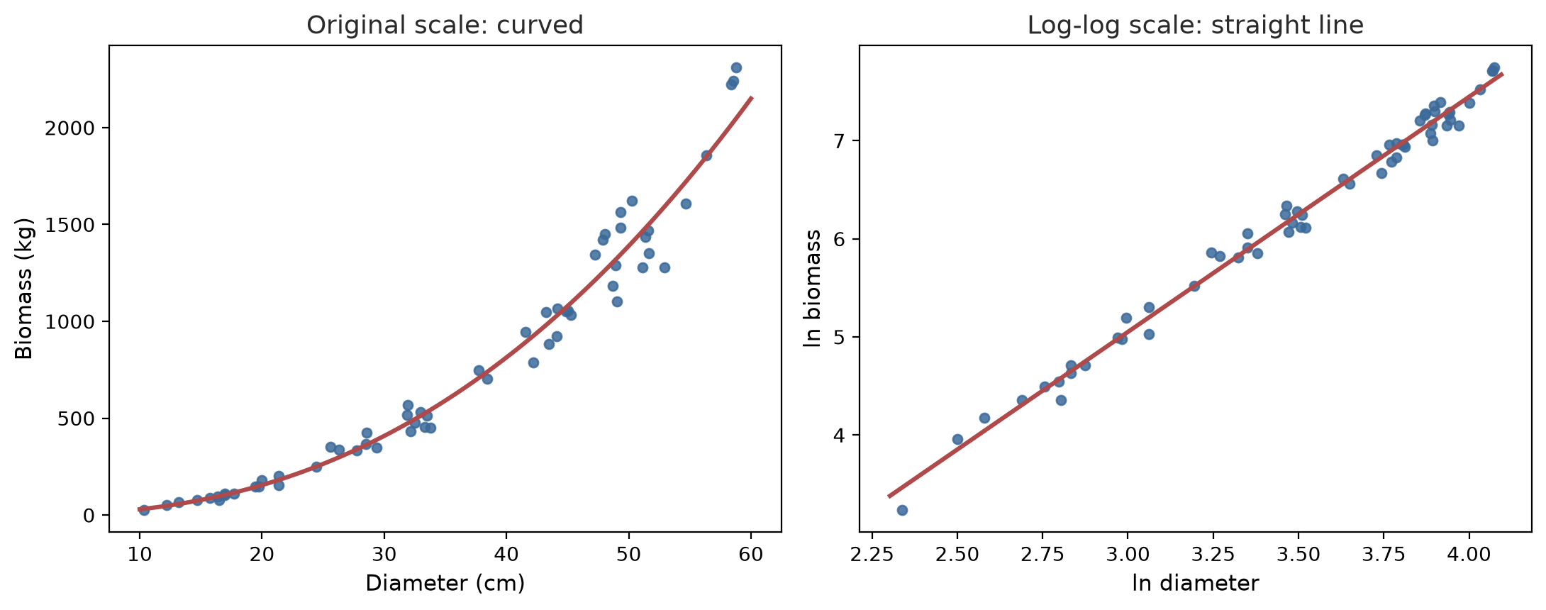
Weighing the biomass of a tree means felling it. Foresters prefer to measure the diameter (easy) and predict biomass with an allometric equation. The relationship curves (a tree twice as thick is far more than twice as heavy), but if both sides are put through a log, it becomes a straight line: ln(biomass) = a + b × ln(diameter).
01_ols_allometric.py
# Chapter 27 - Simple linear regression: a tree allometric equation
import numpy as np
import pandas as pd
import statsmodels.formula.api as smf

rng = np.random.default_rng(42)
n = 60
diameter = rng.uniform(10, 60, n)                                   # cm
biomass = 0.12 * diameter ** 2.4 * np.exp(rng.normal(0, 0.15, n))   # kg (fictional)
trees = pd.DataFrame({"diameter_cm": diameter, "biomass_kg": biomass})
trees["ln_d"] = np.log(trees["diameter_cm"])
trees["ln_b"] = np.log(trees["biomass_kg"])

# The true relationship curves; after taking logs it becomes a straight line
model = smf.ols("ln_b ~ ln_d", data=trees).fit()
print(model.params.round(3))
print("R squared       :", round(model.rsquared, 3))
print("95% interval ln_d:", model.conf_int().loc["ln_d"].round(3).tolist())
print("p-value ln_d    :", format(model.pvalues["ln_d"], ".1e"))

# Predict the biomass of a 40 cm tree (transform back from the log scale)
a, b = model.params["Intercept"], model.params["ln_d"]
correction = np.exp(model.mse_resid / 2)        # bias correction after the log
print()
print("Prediction without correction:", round(np.exp(a) * 40 ** b, 1), "kg")
print("Prediction with correction   :", round(np.exp(a) * 40 ** b * correction, 1), "kg")

# Compare with a straight line fitted directly on the original scale
straight = smf.ols("biomass_kg ~ diameter_cm", data=trees).fit()
print("R squared of the direct straight line:", round(straight.rsquared, 3))
print("Straight-line prediction at 5 cm     :", round(straight.predict(pd.DataFrame({"diameter_cm": [5]}))[0], 1), "kg (nonsense: it can go negative)")
Intercept -2.140
ln_d 2.397
dtype: float64
R squared : 0.99
95% interval ln_d: [2.333, 2.461]
p-value ln_d : 1.9e-59
Prediction without correction: 813.5 kg
Prediction with correction : 818.8 kg
R squared of the direct straight line: 0.908
Straight-line prediction at 5 cm : -501.4 kg (nonsense: it can go negative)- The formula
"ln_b ~ ln_d"reads “ln_b explained by ln_d”.smf.ols(...).fit()finds the line that minimises the sum of squared differences (the least squares method, ordinary least squares, OLS). - The slope b = 2.397 with a 95% interval of 2.333 to 2.461. We planted 2.4 in the data, and the model found it again. When diameter rises by 1%, biomass rises by about 2.4%.
- R squared = 0.99: about 99% of the variation in ln(biomass) is explained by ln(diameter). A high R squared does not guarantee a correct model; it only shows the fit to this data.
- Predicting back to kilograms needs
np.exp, and because the mean of logs is not the log of the mean, there is a small bias correction: 813.5 kg without correction, 818.8 kg with it (factorexp(residual variance / 2)). - A straight line fitted directly on the original scale reaches only an R squared of 0.908 and predicts -501.4 kg for a 5 cm tree: negative mass. The choice of model shape matters.
Multiple regression and diagnostics
Fish weight depends on many things at once. Multiple regression puts several predictors in one model; each coefficient means “the effect of that variable when the others are held fixed”.
02_ols_multiple.py
# Chapter 27 - Multiple regression and diagnostics: fish growth versus feed
import numpy as np
import pandas as pd
import statsmodels.api as sm
import statsmodels.formula.api as smf
from scipy import stats
from statsmodels.stats.diagnostic import het_breuschpagan
from statsmodels.stats.outliers_influence import variance_inflation_factor

rng = np.random.default_rng(42)
n = 80
feed = rng.uniform(20, 60, n)                          # grams of feed per fish per day
temp = rng.normal(28, 1.5, n)                          # degrees Celsius
density = rng.uniform(10, 40, n)                       # fish per m3
weight = 50 + 6.0 * feed + 12 * (temp - 28) - 2.5 * density + rng.normal(0, 25, n)
fish = pd.DataFrame({"weight_g": weight, "feed_g": feed, "temp_c": temp, "density": density})

model = smf.ols("weight_g ~ feed_g + temp_c + density", data=fish).fit()
print(model.summary().tables[1])
print("R squared:", round(model.rsquared, 3), " adjusted R squared:", round(model.rsquared_adj, 3))

# Diagnostic 1: are the residuals normally distributed?
print()
print("Shapiro residuals p   :", round(stats.shapiro(model.resid).pvalue, 3))
# Diagnostic 2: is the residual variance the same at every level? (homoskedasticity)
print("Breusch-Pagan p       :", round(het_breuschpagan(model.resid, model.model.exog)[1], 3))

# Diagnostic 3: multicollinearity (VIF). Add a twin feed that is almost the same
fish["pellet_feed_g"] = 0.9 * fish["feed_g"] + rng.normal(0, 1.5, n)
X = sm.add_constant(fish[["feed_g", "temp_c", "density", "pellet_feed_g"]])
print()
for i, name in enumerate(X.columns):
    if name != "const":
        print(f"VIF {name:14}: {variance_inflation_factor(X.values, i):6.1f}")
==============================================================================
coef std err t P>|t| [0.025 0.975]
------------------------------------------------------------------------------
Intercept -336.0406 61.612 -5.454 0.000 -458.751 -213.330
feed_g 5.9493 0.282 21.133 0.000 5.389 6.510
temp_c 13.8181 2.183 6.330 0.000 9.470 18.166
density -2.4164 0.325 -7.436 0.000 -3.064 -1.769
==============================================================================
R squared: 0.888 adjusted R squared: 0.883
Shapiro residuals p : 0.804
Breusch-Pagan p : 0.746
VIF feed_g : 43.4
VIF temp_c : 1.0
VIF density : 1.0
VIF pellet_feed_g : 43.4- The coefficient table: each gram of feed adds 5.95 g of weight; each degree of temperature adds 13.8 g; each extra fish per m3 subtracts 2.42 g. The values we planted: 6, 12, and -2.5. The confidence interval (the last two columns) and p-value (
P>|t|) are given for every row.0.000means below 0.0005. - Adjusted R squared (0.883) penalises adding useless variables; use it to compare models with different numbers of variables.
- Diagnostics check whether the regression assumptions are reasonable. (1) The residuals (the differences between data and model) should be roughly normal: Shapiro p = 0.804, no sign of violation. (2) The residual variance should be the same at all levels (homoskedasticity): Breusch-Pagan p = 0.746, fine. (3) The predictors should not be too much alike (multicollinearity).
- VIF (variance inflation factor) measures that. We add
pellet_feed_g, an almost-twin offeed_g, and the VIF of both jumps to 43.4 (rough rule: above 5 to 10 is worrying), while temperature and density stay at 1.0. As a result the coefficients of each twin become unstable. The cure: drop one, combine them, or use regularisation (next section).
TipTIP
Always plot the residuals against the predicted values. A curved pattern means the model shape is wrong; a funnel pattern (widening) means unequal variance. Diagnostics are not a formality: a model whose assumptions are broken gives misleading confidence intervals.
Logistic regression: a yes-or-no outcome
When only two outcomes are predicted (tree alive or dead, animal sick or healthy), a straight line would predict “probabilities” below 0 or above 1. Logistic regression predicts a probability (always between 0 and 1) through an S-shaped curve.
03_logistic.py
# Chapter 27 - Logistic regression: the probability a tree survives
import numpy as np
import pandas as pd
import statsmodels.formula.api as smf

rng = np.random.default_rng(42)
n = 200
diameter = rng.uniform(5, 50, n)
plot = rng.choice(["A", "B", "C"], n)
logit = -2.5 + 0.12 * diameter + np.where(plot == "C", -0.8, 0)
alive = rng.random(n) < 1 / (1 + np.exp(-logit))
trees = pd.DataFrame({"alive": alive.astype(int), "diameter_cm": diameter, "plot": plot})

model = smf.logit("alive ~ diameter_cm + C(plot)", data=trees).fit(disp=False)
print(model.params.round(3))

# Coefficients are on the log-odds scale; turn them into odds ratios
print()
print("Odds ratios (OR):")
print(np.exp(model.params).round(3))
print("Each extra 1 cm of diameter multiplies the survival odds by", round(np.exp(model.params["diameter_cm"]), 3))

# Probability for new trees
new = pd.DataFrame({"diameter_cm": [10, 30], "plot": ["A", "A"]})
print()
print("Survival probability (diameter 10 and 30 cm, plot A):", model.predict(new).round(3).tolist())

# Accuracy with a threshold of 0.5
predicted = (model.predict(trees) >= 0.5).astype(int)
print("Accuracy:", round((predicted == trees["alive"]).mean(), 3))
print("True proportion alive:", round(trees["alive"].mean(), 3))
Intercept -2.385
C(plot)[T.B] -0.084
C(plot)[T.C] -0.487
diameter_cm 0.107
dtype: float64
Odds ratios (OR):
Intercept 0.092
C(plot)[T.B] 0.919
C(plot)[T.C] 0.614
diameter_cm 1.113
dtype: float64
Each extra 1 cm of diameter multiplies the survival odds by 1.113
Survival probability (diameter 10 and 30 cm, plot A): [0.211, 0.693]
Accuracy: 0.77
True proportion alive: 0.555- The coefficients are on the log-odds scale, hard to read directly.
np.exp(coefficient)turns them into odds ratios (OR): each extra 1 cm of diameter multiplies the survival odds by 1.113 (up about 11%). Plot C has an OR of 0.614: lower survival odds, as we planted. - Odds = probability / (1 - probability). A probability of 0.5 equals odds of 1. Odds and probability are not the same thing, so do not say “11% more likely” for a probability.
predictgives probabilities: a 10 cm tree in plot A about 0.211 and a 30 cm tree about 0.693.- With a threshold of 0.5, accuracy is 0.77, better than guessing “all alive” (true proportion alive 0.555). For imbalanced cases (a rare disease), accuracy alone misleads; check precision and recall too, in Series A3.
GLM: count data with Poisson
The number of fruits per tree, the number of eggs, or the number of fallen trees are non-negative whole numbers. A GLM (generalized linear model) extends regression to other families of distributions. For counts, the Poisson family with a log link is used.
04_glm_poisson.py
# Chapter 27 - Poisson GLM for count data: number of fruits per tree
import numpy as np
import pandas as pd
import statsmodels.api as sm
import statsmodels.formula.api as smf

rng = np.random.default_rng(42)
n = 150
diameter = rng.uniform(10, 50, n)
mu = np.exp(0.5 + 0.06 * diameter)
mean = mu * rng.gamma(shape=4, scale=0.25, size=n)   # extra variation between trees
fruits = rng.poisson(mean)
data = pd.DataFrame({"fruits": fruits, "diameter_cm": diameter})

poisson = smf.glm("fruits ~ diameter_cm", data=data, family=sm.families.Poisson()).fit()
print(poisson.params.round(4))
print("Rate ratio (IRR) per cm:", round(np.exp(poisson.params["diameter_cm"]), 4))

# Check overdispersion: Pearson chi-square divided by degrees of freedom; ideally about 1
dispersion = poisson.pearson_chi2 / poisson.df_resid
print("Dispersion:", round(dispersion, 2), "(far above 1 means Poisson is too optimistic)")

# Alternative: negative binomial, which estimates the extra variation (alpha) itself
nb = smf.negativebinomial("fruits ~ diameter_cm", data=data).fit(disp=False)
print()
print("Negative binomial, alpha :", round(nb.params["alpha"], 3))
print("SE diameter Poisson      :", round(poisson.bse["diameter_cm"], 5))
print("SE diameter neg. binomial:", round(nb.bse["diameter_cm"], 5))
Intercept 0.6400
diameter_cm 0.0577
dtype: float64
Rate ratio (IRR) per cm: 1.0594
Dispersion: 4.64 (far above 1 means Poisson is too optimistic)
Negative binomial, alpha : 0.267
SE diameter Poisson : 0.00234
SE diameter neg. binomial: 0.00477exp(0.0577)= 1.0594: each extra 1 cm of diameter raises the average number of fruits by about 5.9% (the rate ratio, IRR).- Poisson assumes variance = mean. Real data is often more variable (overdispersion). The measure: Pearson chi-square divided by the degrees of freedom. Here it is 4.64, far above 1. As a result the Poisson standard errors are too small and the conclusions too confident.
- The negative binomial estimates the extra variation itself (
alpha= 0.267). The standard error of diameter becomes 0.00477, almost double the 0.00234 of Poisson. That is the price of honesty.
Ridge and Lasso: when predictors are many and alike
With many mutually related predictors, OLS estimates wild coefficients (positive in one place, negative in another) and overfits: good on training data, poor on new data. Regularisation adds a “penalty” for large coefficients. Ridge shrinks all coefficients; Lasso shrinks and can set some to zero, selecting variables at the same time.
05_ridge_lasso.py
# Chapter 27 - Regularisation (Ridge and Lasso): cattle weight from many body measurements
import numpy as np
from sklearn.linear_model import LassoCV, LinearRegression, RidgeCV
from sklearn.model_selection import train_test_split
from sklearn.pipeline import make_pipeline
from sklearn.preprocessing import StandardScaler

rng = np.random.default_rng(42)
n, p = 90, 10
base = rng.normal(size=(n, 1))
# 10 closely related measurements; only 3 truly matter
X = base + rng.normal(0, 0.5, size=(n, p))
true_coef = np.array([30, 20, 10, 0, 0, 0, 0, 0, 0, 0])
weight = 350 + X @ true_coef / 3 + rng.normal(0, 15, n)   # kg (fictional)

X_train, X_test, y_train, y_test = train_test_split(X, weight, test_size=0.3, random_state=42)

models = {
    "Plain OLS": make_pipeline(StandardScaler(), LinearRegression()),
    "Ridge": make_pipeline(StandardScaler(), RidgeCV(alphas=np.logspace(-2, 3, 30))),
    "Lasso": make_pipeline(StandardScaler(), LassoCV(cv=5, random_state=42)),
}
for name, m in models.items():
    m.fit(X_train, y_train)
    coef = m[-1].coef_
    print(f"{name:10} test R2 = {m.score(X_test, y_test):.3f}   zero coefficients: {int((np.abs(coef) < 1e-9).sum())} of {p}")
    print("           ", np.round(coef, 1) + 0.0)
Plain OLS test R2 = 0.680 zero coefficients: 0 of 10
[12.9 0.5 -4.8 6.5 -1.8 -0.4 3.6 2. 2.5 -0.4]
Ridge test R2 = 0.754 zero coefficients: 0 of 10
[ 8.5 2.2 -2. 4.3 -1.1 0.6 2.5 2.1 2.5 0.6]
Lasso test R2 = 0.724 zero coefficients: 5 of 10
[12.2 0. 0. 3.2 0. 0. 1.5 0.7 1.9 0. ]We set aside 30% of the data as test data that the model never sees while learning. Test R squared: OLS 0.680, Lasso 0.724, Ridge 0.754. The OLS coefficients are all over the place (12.9, 0.5, -4.8, …), Ridge is calmer, and Lasso zeroes 5 of 10. The predictors are put on one scale first (StandardScaler) because the penalty depends on scale. The size of the penalty is chosen automatically by cross-validation (RidgeCV, LassoCV).
WarningWARNING
The score on training data is always too good. A model’s value is honest only when tested on data not used to build it. This principle recurs throughout Series A3.
Non-linear regression: growth curves
Fish do not grow in a straight line forever; they approach a maximum length. The von Bertalanffy curve describes this: L(t) = Lmax × (1 - e^(-k (t - t0))). Its parameters are not linear coefficients, so we use curve_fit, which searches for the best values step by step, starting from an initial guess p0.
06_nonlinear.py
# Chapter 27 - Non-linear regression: fish growth curve (von Bertalanffy)
import numpy as np
from scipy.optimize import curve_fit


def length(age, l_max, k, t0):
    """Fish length (cm) at a given age (months)."""
    return l_max * (1 - np.exp(-k * (age - t0)))


rng = np.random.default_rng(42)
age = np.linspace(1, 24, 30)
true = length(age, l_max=45, k=0.15, t0=-0.5)
measured = true + rng.normal(0, 1.2, age.size)       # measured length with error

estimate, covariance = curve_fit(length, age, measured, p0=[40, 0.1, 0])
error = np.sqrt(np.diag(covariance))
for name, value, se in zip(["l_max", "k", "t0"], estimate, error):
    print(f"{name:7} = {value:7.3f}  (standard error {se:.3f})")

residual = measured - length(age, *estimate)
print("Root mean squared residual:", round(float(np.sqrt((residual ** 2).mean())), 3), "cm")
print("Predicted length at 12 months:", round(float(length(12, *estimate)), 1), "cm")
print("Predicted length at 36 months:", round(float(length(36, *estimate)), 1), "cm (close to l_max)")
l_max = 45.405 (standard error 0.521)
k = 0.146 (standard error 0.007)
t0 = -0.484 (standard error 0.165)
Root mean squared residual: 0.899 cm
Predicted length at 12 months: 38.1 cm
Predicted length at 36 months: 45.2 cm (close to l_max)Estimates: Lmax = 45.405 cm (standard error 0.521), k = 0.146 per month (0.007), t0 = -0.484. The values we planted: 45, 0.15, and -0.5, so all three are found again within the range of the standard errors. The prediction at 36 months (45.2 cm) approaches Lmax: the curve flattens. The standard errors come from the covariance matrix returned by curve_fit.
WarningWARNING
Non-linear curves can be very sensitive to the initial guess p0 and can fail to converge. Draw the curve over the data before trusting it. Do not predict far outside the range of the data (extrapolation): the model only knows what it has seen.
Mixed-effects models: grouped data
Cattle in the same pen are not independent: they share feed, cleanliness, and a keeper. Treating them all as independent (plain OLS) deceives the standard errors. A mixed-effects model adds a random effect per group (pen) next to the fixed effect we want to know (feed).
07_mixed_effects.py
# Chapter 27 - Mixed-effects model: cattle in many pens
import numpy as np
import pandas as pd
import statsmodels.formula.api as smf

rng = np.random.default_rng(42)
rows = []
for pen in range(1, 9):
    pen_effect = rng.normal(0, 12)              # each pen has its own fortune
    for _ in range(10):
        feed = rng.uniform(8, 14)               # kg of feed per day
        gain = 20 + 6 * feed + pen_effect + rng.normal(0, 8)
        rows.append({"pen": f"K{pen}", "feed_kg": feed, "weight_gain_kg": gain})
cattle = pd.DataFrame(rows)

plain = smf.ols("weight_gain_kg ~ feed_kg", data=cattle).fit()
mixed = smf.mixedlm("weight_gain_kg ~ feed_kg", data=cattle, groups=cattle["pen"]).fit()

print("Plain OLS     : feed coef =", round(plain.params["feed_kg"], 3), " standard error =", round(plain.bse["feed_kg"], 3))
print("Mixed effects : feed coef =", round(mixed.params["feed_kg"], 3), " standard error =", round(mixed.bse["feed_kg"], 3))

pen_variance = float(mixed.cov_re.iloc[0, 0])
resid_variance = float(mixed.scale)
print("Between-pen variance:", round(pen_variance, 1))
print("Residual variance   :", round(resid_variance, 1))
print("ICC (share of variation due to the pen):", round(pen_variance / (pen_variance + resid_variance), 3))
print()
print("Random effect per pen (difference from the average):")
print(pd.Series({k: round(float(v.iloc[0]), 1) for k, v in mixed.random_effects.items()}).to_string())
Plain OLS : feed coef = 5.131 standard error = 0.772
Mixed effects : feed coef = 5.635 standard error = 0.476
Between-pen variance: 103.0
Residual variance : 47.9
ICC (share of variation due to the pen): 0.683
Random effect per pen (difference from the average):
K1 6.5
K2 -5.7
K3 -8.0
K4 7.5
K5 -14.9
K6 -2.6
K7 16.3
K8 1.0- Plain OLS estimates the effect of feed at 5.131 (standard error 0.772); the mixed model 5.635 (0.476). The value we planted was 6. The mixed model separates “the pen’s fortune” from the noise, so it is more precise.
- Between-pen variance 103.0 and residual variance 47.9. The ICC (intraclass correlation) = 103.0 / (103.0 + 47.9) = 0.683: about 68% of the variation in weight gain comes from differences between pens. That is large: ignoring the pen is a serious mistake.
- The random effect per pen shows K7 (+16.3) as the luckiest and K5 (-14.9) as the unluckiest, relative to the average.
Mixed models are the standard tool for nested plots in a forest, ponds within a farm, or repeated measurements on the same tree.
Time series and forecasting with ARIMA
Data measured in sequence over time (monthly rainfall) has a memory: this month resembles last month, and there is a seasonal pattern. ARIMA models that through three parts: AR (past values explain the present value), I (differencing to flatten a trend), MA (past errors also have an influence). seasonal_order=(P, D, Q, 12) adds a pattern that repeats every 12 months.
08_arima.py
# Chapter 27 - Time series and forecasting with ARIMA: monthly rainfall
import numpy as np
import pandas as pd
from statsmodels.tsa.arima.model import ARIMA

rng = np.random.default_rng(42)
months = pd.period_range("2019-01", periods=72, freq="M")
season = 120 + 70 * np.cos(2 * np.pi * (np.arange(72) - 1) / 12)       # yearly pattern
rain = pd.Series(season + rng.normal(0, 18, 72), index=months).clip(lower=0).round(1)  # mm (fictional)

train, test = rain[:60], rain[60:]          # keep the last 12 months to test the forecast

model = ARIMA(train, order=(1, 0, 0), seasonal_order=(1, 1, 0, 12)).fit()
forecast = model.forecast(steps=12)

mae = (test - forecast).abs().mean()
# Simple benchmark: this month equals the same month last year
naive = pd.Series(train.values[-12:], index=test.index)
mae_naive = (test - naive).abs().mean()
print("MAE of the seasonal ARIMA forecast:", round(mae, 1), "mm")
print("MAE of the seasonal naive benchmark:", round(mae_naive, 1), "mm")
print()
print(pd.DataFrame({"actual": test, "forecast": forecast.round(1)}).head(6))
MAE of the seasonal ARIMA forecast: 15.0 mm
MAE of the seasonal naive benchmark: 17.8 mm
actual forecast
2024-01 150.3 187.5
2024-02 184.0 185.1
2024-03 183.6 178.4
2024-04 165.6 166.5
2024-05 132.8 108.5
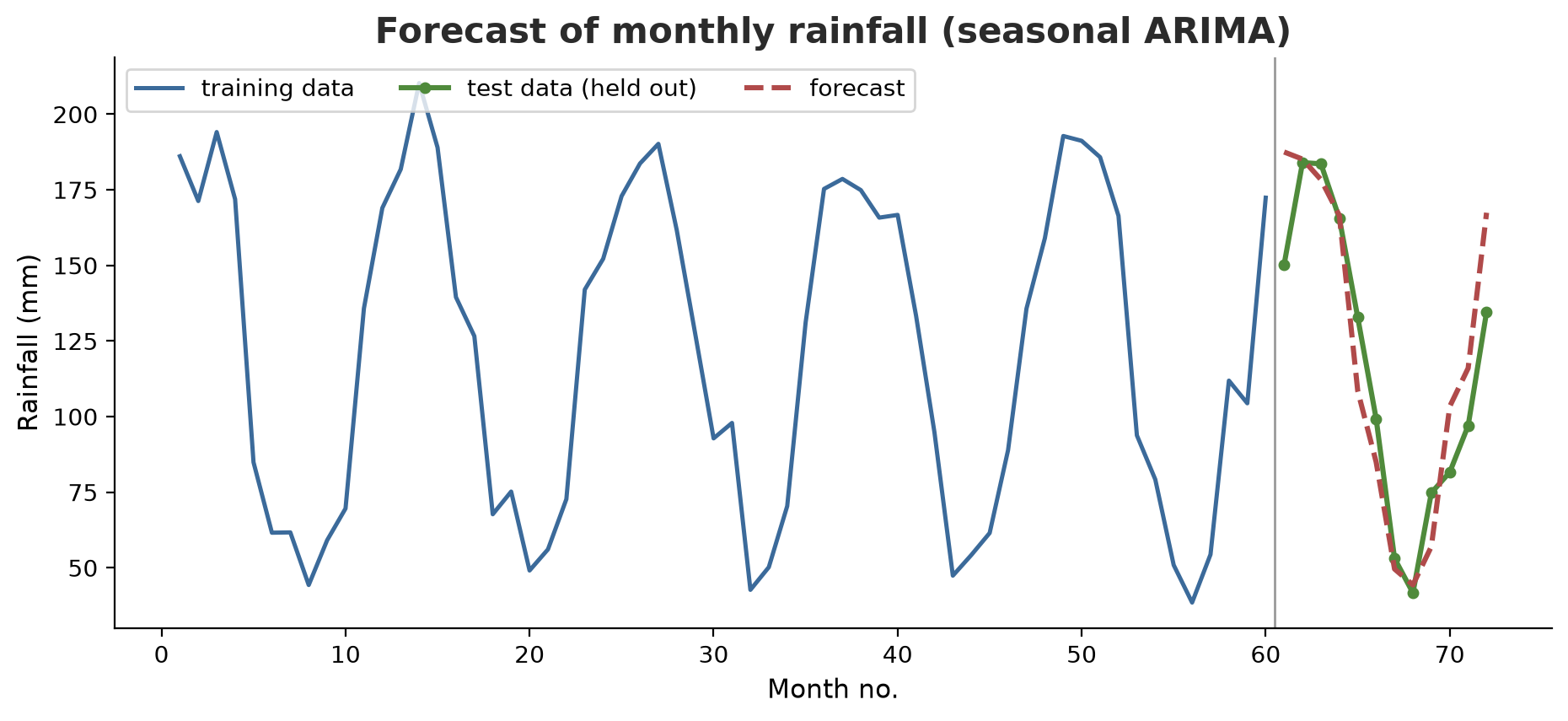
2024-06 99.3 85.0- We keep the last 12 months as an exam and forecast them from the 60 months before. That is the honest way to test a forecast.
- The simple benchmark (“this month = the same month last year”) misses by 17.8 mm on average; seasonal ARIMA by 15.0 mm. A complicated model must always be compared with a simple benchmark; if it does not win by a clear margin, use the simple one.
- The table shows the first six months: the forecast follows the season, but does not capture the random noise of each month (January: 187.5 forecast vs 150.3 actual). A forecast gives a pattern, not certainty.
Spatial regression: GWR
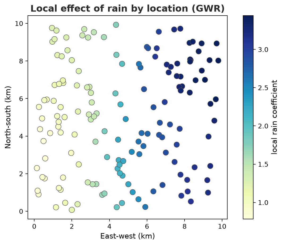
Ordinary regression gives one coefficient for the whole region. Yet the effect of rain on harvest can differ on the western and eastern slopes. GWR (geographically weighted regression) runs many local regressions, each location with its own coefficient, weighting near neighbours more heavily. The mgwr library does the job.
09_gwr.py
# Chapter 27 - Spatial regression: GWR (geographically weighted regression) with mgwr
import numpy as np
import statsmodels.api as sm
from mgwr.gwr import GWR
from mgwr.sel_bw import Sel_BW

rng = np.random.default_rng(42)
n = 150
# Coordinates of 150 orchard plots in a 10 x 10 km area (fictional)
coords = rng.uniform(0, 10, size=(n, 2))
rain = rng.normal(0, 1, size=(n, 1))                   # standardised rainfall
# The effect of rain strengthens from west (x = 0) to east (x = 10)
effect = 0.5 + 0.35 * coords[:, [0]]
yield_t = 5 + effect * rain + rng.normal(0, 0.4, size=(n, 1))   # tonnes/ha (fictional)

# Global model: a single coefficient for the whole area
global_ols = sm.OLS(yield_t, sm.add_constant(rain)).fit()
print("Global OLS: rain coefficient =", round(float(global_ols.params[1]), 3), " R2 =", round(float(global_ols.rsquared), 3))

# GWR: a different coefficient at every location
bandwidth = Sel_BW(coords, yield_t, rain).search()
result = GWR(coords, yield_t, rain, bandwidth).fit()
local = result.params[:, 1]
print("Chosen bandwidth (number of neighbours):", int(bandwidth))
print("GWR: R2 =", round(float(result.R2), 3))
print("Local rain coefficient: min =", round(float(local.min()), 2), " max =", round(float(local.max()), 2))

west = coords[:, 0] < 3
east = coords[:, 0] > 7
print("Mean coefficient in the west (x < 3):", round(float(local[west].mean()), 2))
print("Mean coefficient in the east (x > 7):", round(float(local[east].mean()), 2))
print("True effect in the west/east        :", round(float(effect[west].mean()), 2), "/", round(float(effect[east].mean()), 2))
Global OLS: rain coefficient = 2.176 R2 = 0.788
Chosen bandwidth (number of neighbours): 46
GWR: R2 = 0.97
Local rain coefficient: min = 0.78 max = 3.44
Mean coefficient in the west (x < 3): 1.09
Mean coefficient in the east (x > 7): 3.26
True effect in the west/east : 1.01 / 3.41- This script uses
mgwr, an extra library outside the basic packages of this chapter; install it withpip install mgwr(it bringslibpysal,spreg, andspglmalong). On the author’s computer, the library was available as a ready-made package for Python 3.14 and this script was really run. - Global OLS estimates a single rain coefficient of 2.176 (R squared 0.788). GWR finds local coefficients from 0.78 to 3.44: weak in the west (average 1.09) and strong in the east (3.26), close to the values we planted (1.01 and 3.41). One global number hides this pattern.
Sel_BWchooses the bandwidth (here 46 nearest neighbours) through an automatic search. A narrow window = very local but noisy; a wide one = smooth but less sensitive.- Careful: the GWR R squared of 0.97 is computed on the same data used for estimation, and GWR is far more flexible than OLS, so that figure must not simply be compared with 0.788. Use criteria such as AICc or test data. The coordinates here are fictional; real map data and projections are covered in the geospatial series.
Monte Carlo simulation: computing uncertainty
Yield, price, and cost are uncertain. Instead of a single profit figure, we draw the input values hundreds of thousands of times from plausible distributions, compute the profit each time, and look at the distribution of profit. This is Monte Carlo (named after the casino, because of the “drawing”).
10_monte_carlo.py
# Chapter 27 - Monte Carlo simulation: uncertainty in maize harvest income
import numpy as np

rng = np.random.default_rng(42)
N = 100_000
area_ha = 2.0

# Every input is uncertain, so we draw from plausible distributions (fictional example numbers)
yield_t_ha = rng.triangular(left=3.0, mode=5.0, right=6.5, size=N)     # harvest yield
price_rp_kg = rng.normal(loc=5000, scale=700, size=N)                  # selling price
cost_rp = rng.normal(loc=40_000_000, scale=3_000_000, size=N)          # total cost

income = yield_t_ha * 1000 * area_ha * price_rp_kg
profit = income - cost_rp

print("Mean profit (million Rp):", round(profit.mean() / 1e6, 2))
print("Standard deviation (million Rp):", round(profit.std() / 1e6, 2))
print("90% interval of profit (million Rp):", np.percentile(profit, [5, 95]).round(-4) / 1e6)
print("Probability of a loss    :", round(float((profit < 0).mean()), 3))

# How many draws are enough? Compare a few sizes
for n in (100, 1000, 100_000):
    print(f"  loss probability estimated from {n:>7} draws:", round(float((profit[:n] < 0).mean()), 3))
Mean profit (million Rp): 8.36
Standard deviation (million Rp): 10.34
90% interval of profit (million Rp): [-8.03 25.96]
Probability of a loss : 0.216
loss probability estimated from 100 draws: 0.21
loss probability estimated from 1000 draws: 0.224
loss probability estimated from 100000 draws: 0.216The mean profit is 8.36 million rupiah, but its standard deviation is 10.34 million: the uncertainty is large. The 90% interval of profit: from -8.03 to 25.96 million. The probability of a loss is 21.6%. A single average hides this risk. The last three lines show the estimated loss probability settling around 0.2 after thousands of draws; 100 draws is too few for a tidy number. All numbers (yield, price, cost) are fictional examples, not real prices or advice.
Optimisation: finding the best choice
scipy.optimize solves two common kinds of problem. Linear programming (linprog): minimise cost subject to linear equalities and inequalities. One-variable optimisation (minimize_scalar): find the highest or lowest point of a function.
11_optimization.py
# Chapter 27 - Optimisation with scipy.optimize: the cheapest feed mix
from scipy.optimize import linprog, minimize_scalar

# Two ingredients: maize (Rp 5,000/kg, 8% protein) and soybean meal (Rp 9,000/kg, 44% protein)
# Requirement: 100 kg of mix with at least 18% protein. Fictional example numbers.
cost = [5000, 9000]
# linprog wants the "less than" form: -(protein) <= -(requirement)
protein_a = [[-0.08, -0.44]]
protein_b = [-0.18 * 100]
total_a = [[1, 1]]
total_b = [100]

result = linprog(cost, A_ub=protein_a, b_ub=protein_b,
                 A_eq=total_a, b_eq=total_b, bounds=[(0, None), (0, None)])
print("Success?        :", result.success)
print("Maize (kg)      :", round(result.x[0], 2))
print("Soybean (kg)    :", round(result.x[1], 2))
print("Cost (Rp)       :", round(result.fun))

# One-variable optimisation: the fish stocking density that maximises profit (fictional model)
def negative_profit(density):
    final_weight = 900 * (1 - density / 120)       # weight shrinks when too crowded
    return -(density * final_weight / 1000 * 25000 - density * 800)

search = minimize_scalar(negative_profit, bounds=(1, 100), method="bounded")
print()
print("Best stocking density (fish/m2):", round(search.x, 1))
print("Maximum profit (Rp/m2)         :", round(-search.fun))
Success? : True
Maize (kg) : 72.22
Soybean (kg) : 27.78
Cost (Rp) : 611111
Best stocking density (fish/m2): 57.9
Maximum profit (Rp/m2) : 627853- A 100 kg feed mix with at least 18% protein uses 72.22 kg of maize and 27.78 kg of soybean meal, at a cost of Rp 611,111. Soybean meal is pricier but rich in protein; the solver finds the cheapest mix that meets the requirement.
linprogonly accepts the “less than or equal” form, so the “minimum protein” requirement is written with a minus sign. - The second problem: the stocking density that maximises profit is 57.9 fish/m2. Too sparse wastes the pond; too crowded stunts the fish. The optimum lies in the middle. The model is deliberately simple and fictional.
System dynamics models and sensitivity analysis
Systems that change over time (a fish stock, a forest stand) are often written as equations of rate of change. The logistic model says the stock grows by r × stock × (1 - stock / K) (K = carrying capacity), minus the harvest. solve_ivp computes the journey step by step.
12_system_dynamics.py
# Chapter 27 - System dynamics and sensitivity analysis: fish stock in a small reservoir
import numpy as np
from scipy.integrate import solve_ivp


def final_stock(r=0.8, K=1000.0, harvest=100.0, start=300.0, years=10):
    """Logistic population with a fixed harvest per year (tonnes, fictional numbers)."""
    def rate(t, y):
        return [r * y[0] * (1 - y[0] / K) - harvest]
    extinct = lambda t, y: y[0]       # event: the stock touches zero
    extinct.terminal = True
    sol = solve_ivp(rate, (0, years), [start], events=extinct, t_eval=[years])
    return 0.0 if sol.status == 1 else float(sol.y[0, -1])


baseline = final_stock()
print("Stock after 10 years (baseline case):", round(baseline, 1), "tonnes")

# One-at-a-time sensitivity analysis: change each parameter by +-20%
print()
print(f"{'parameter':10} {'-20%':>8} {'+20%':>8} {'range':>9}")
for name in ("r", "K", "harvest", "start"):
    values = dict(r=0.8, K=1000.0, harvest=100.0, start=300.0)
    low = final_stock(**{**values, name: values[name] * 0.8})
    high = final_stock(**{**values, name: values[name] * 1.2})
    print(f"{name:10} {low:8.1f} {high:8.1f} {abs(high - low):9.1f}")

# Tipping point: which harvest is still sustainable?
for harvest in (100, 150, 190, 210):
    print(f"harvest {harvest} tonnes/year -> final stock {final_stock(harvest=harvest):7.1f} tonnes")
Stock after 10 years (baseline case): 844.8 tonnes
parameter -20% +20% range
r 753.3 880.2 126.9
K 636.5 1048.6 412.1
harvest 882.4 798.9 83.5
start 837.7 847.9 10.2
harvest 100 tonnes/year -> final stock 844.8 tonnes
harvest 150 tonnes/year -> final stock 679.6 tonnes
harvest 190 tonnes/year -> final stock 0.0 tonnes
harvest 210 tonnes/year -> final stock 0.0 tonnes- Baseline case: a stock of 300 tonnes rises to 844.8 tonnes after 10 years with a harvest of 100 tonnes per year.
- A sensitivity analysis changes one parameter by ±20% while holding the others, then sees how far the result shifts. The carrying capacity K matters most (range 412.1 tonnes), the rate r moderately (126.9), the harvest little (83.5), and the starting stock hardly at all (10.2) because the stock heads for equilibrium. This result shows which data deserves careful measurement: K.
- Tipping point: a harvest of 150 tonnes/year is still safe (stock 679.6), but 190 tonnes/year destroys the stock (0.0), even though that figure is below the theoretical limit rK/4 = 200 tonnes. The reason: with a harvest of 190 the stock balance equation has two points, about 388 tonnes (unstable) and 612 tonnes (stable). The starting stock of 300 lies below the unstable point, so the stock slides down until it is gone. Real fish stocks can collapse suddenly. That is why system models are useful.
Running Project I3: models for our information system
We bring together the project’s four models: tree allometry, fish weight against feed, cattle weight against feed, and harvest against rainfall. The summarise() function condenses each model into one row.
13_project_regression.py
# Chapter 27 - Running project I3: four models for our information system
import numpy as np
import pandas as pd
import statsmodels.formula.api as smf

rng = np.random.default_rng(42)


def summarise(name, model, variable):
    """One summary row: coefficient, 95% interval, R squared."""
    b = model.params[variable]
    lo, hi = model.conf_int().loc[variable]
    return {"model": name, "variable": variable, "coef": round(b, 3),
            "lower95": round(lo, 3), "upper95": round(hi, 3), "R2": round(model.rsquared, 3)}


# 1. Tree allometry: ln(biomass) ~ ln(diameter)
d = rng.uniform(10, 60, 60)
trees = pd.DataFrame({"ln_d": np.log(d), "ln_b": np.log(0.12 * d ** 2.4 * np.exp(rng.normal(0, 0.15, 60)))})
m1 = smf.ols("ln_b ~ ln_d", data=trees).fit()

# 2. Fish: weight gain (g) ~ feed (g/day)
fish_feed = rng.uniform(20, 60, 50)
fish = pd.DataFrame({"feed": fish_feed, "gain_g": 15 + 4.2 * fish_feed + rng.normal(0, 20, 50)})
m2 = smf.ols("gain_g ~ feed", data=fish).fit()

# 3. Cattle: weight gain (kg) ~ feed (kg/day)
cattle_feed = rng.uniform(8, 14, 40)
cattle = pd.DataFrame({"feed": cattle_feed, "gain_kg": 10 + 5.5 * cattle_feed + rng.normal(0, 7, 40)})
m3 = smf.ols("gain_kg ~ feed", data=cattle).fit()

# 4. Harvest vs rainfall: a humped curve (too dry or too wet both hurt)
rain = rng.uniform(600, 2400, 70)                        # mm per season
harvest = 0.5 + 0.0060 * rain - 0.0000018 * rain ** 2 + rng.normal(0, 0.3, 70)   # tonnes/ha
orchard = pd.DataFrame({"rain": rain, "harvest": harvest})
m4 = smf.ols("harvest ~ rain + I(rain ** 2)", data=orchard).fit()

table = pd.DataFrame([
    summarise("Tree allometry (log scale)", m1, "ln_d"),
    summarise("Fish: weight ~ feed", m2, "feed"),
    summarise("Cattle: weight ~ feed", m3, "feed"),
])
print(table.to_string(index=False))

b1, b2 = m4.params["rain"], m4.params["I(rain ** 2)"]
optimum = -b1 / (2 * b2)
print()
print("Harvest ~ rain + rain^2: R2 =", round(m4.rsquared, 3), " squared-term p =", format(m4.pvalues["I(rain ** 2)"], ".1e"))
print("Optimal rainfall (peak of the curve):", round(optimum), "mm per season")

# Uncertainty of the peak via bootstrap (resampling with replacement)
peaks = []
for _ in range(500):
    s = orchard.sample(len(orchard), replace=True, random_state=int(rng.integers(1_000_000)))
    mb = smf.ols("harvest ~ rain + I(rain ** 2)", data=s).fit()
    peaks.append(-mb.params["rain"] / (2 * mb.params["I(rain ** 2)"]))
print("95% bootstrap interval for the peak:", np.percentile(peaks, [2.5, 97.5]).round().tolist(), "mm")
model variable coef lower95 upper95 R2
Tree allometry (log scale) ln_d 2.397 2.333 2.461 0.990
Fish: weight ~ feed feed 4.210 3.753 4.667 0.877
Cattle: weight ~ feed feed 5.917 4.788 7.045 0.748
Harvest ~ rain + rain^2: R2 = 0.608 squared-term p = 1.6e-10
Optimal rainfall (peak of the curve): 1711 mm per season
95% bootstrap interval for the peak: [1653.0, 1800.0] mm- The table: allometry b = 2.397 (R squared 0.990), fish 4.210 g per gram of feed (0.877), cattle 5.917 kg per kg of feed (0.748). The confidence intervals contain the values we planted (2.4; 4.2; 5.5). The cattle interval is the widest (4.788 to 7.045) because it has the least data (40) and is the noisiest.
- Harvest versus rain has a humped curve: too dry or too wet both hurt. The model
harvest ~ rain + I(rain ** 2)is still linear in its coefficients, so plain OLS is enough. The squared term is highly significant (p = 1.6e-10), R squared 0.608. - The peak of the curve, -b1 / (2 × b2), is at about 1711 mm per season (the value we planted: 1667). The bootstrap (500 resamples with replacement) gives a 95% interval for the peak: 1653 to 1800 mm. Giving an “optimum” number an uncertainty interval is far more honest than a single figure.
All these models go into the Quarto report in Chapter 29.
Exercises
- In
01_ols_allometric.py, predict the biomass of a 25 cm and a 55 cm tree (with bias correction). Why is predicting a 150 cm tree not safe? - In
03_logistic.py, change the diameter coefficient in the data from 0.12 to 0.02. How do the accuracy and the odds ratio change? - In
12_system_dynamics.py, find (by trying several values) the largest harvest for which the stock still survives after 10 years. Compare it with 200 tonnes. - Challenge: create data with one important predictor and five junk predictors, then compare the test R squared of OLS and Lasso. When does Lasso win?
Chapter Summary
- OLS:
smf.ols("y ~ x", data=...); read the coefficients, the 95% interval, R squared. Log-log turns a power relationship into a straight line. - Diagnostics: normal residuals (Shapiro), equal variance (Breusch-Pagan), no twins (VIF).
- Logistic for yes/no (odds ratios), Poisson GLM for counts (check overdispersion), Ridge/Lasso for many predictors (test on test data).
- Non-linear (
curve_fit), mixed effects (mixedlm) for grouped data, ARIMA for time series (test with held-out data), GWR for coefficients that change by location. - Monte Carlo computes uncertainty; optimisation finds the best choice; system dynamics and sensitivity show tipping points and the most influential variables.
- A model is a tool, not the truth: check assumptions, test on new data, and report the uncertainty.
Next, in Chapter 28: qualitative and mixed methods: how to analyse interviews with farmers, fishers, and livestock keepers, and combine them with numbers.